Try the new view →
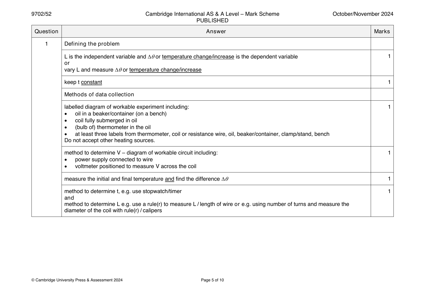
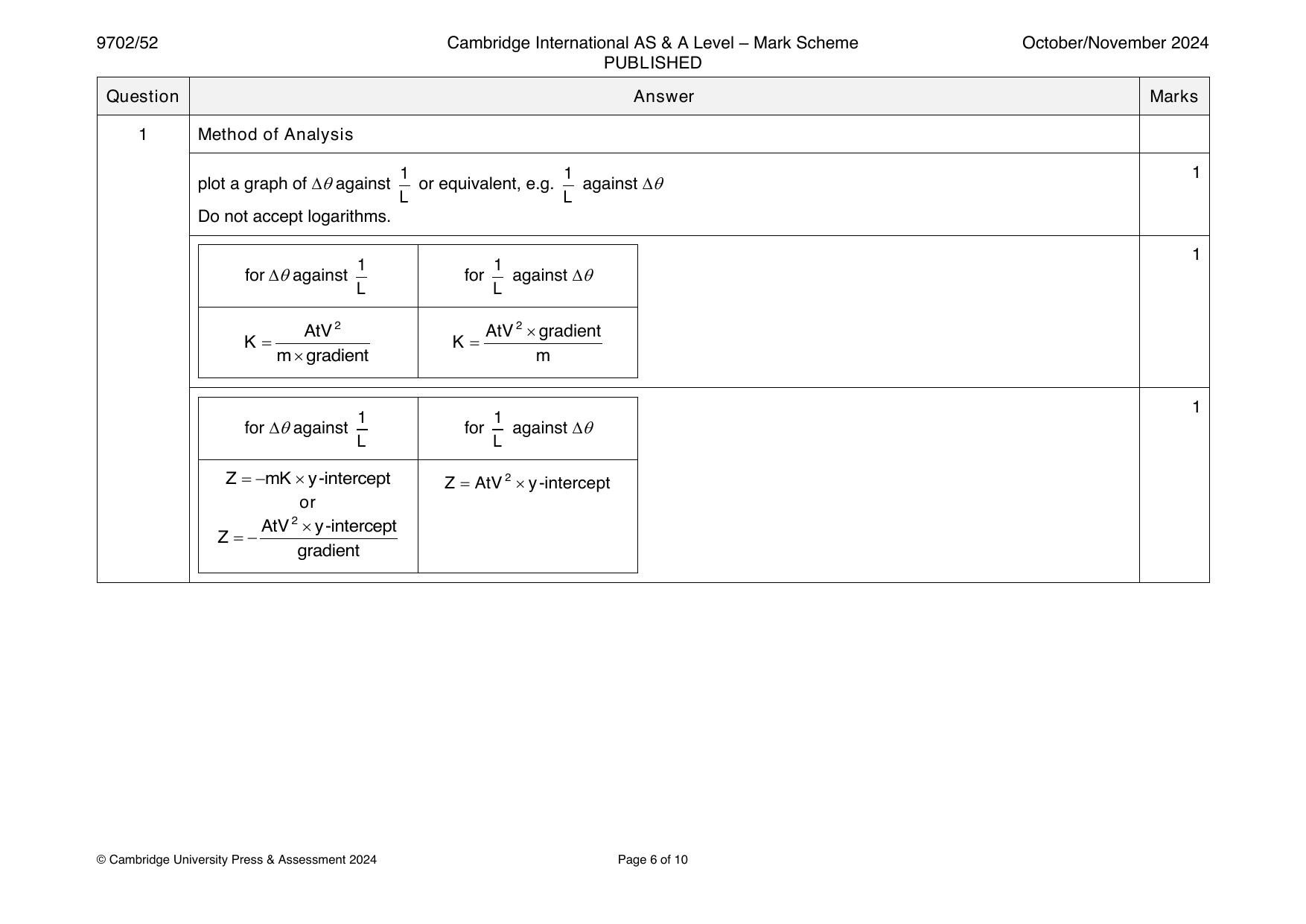
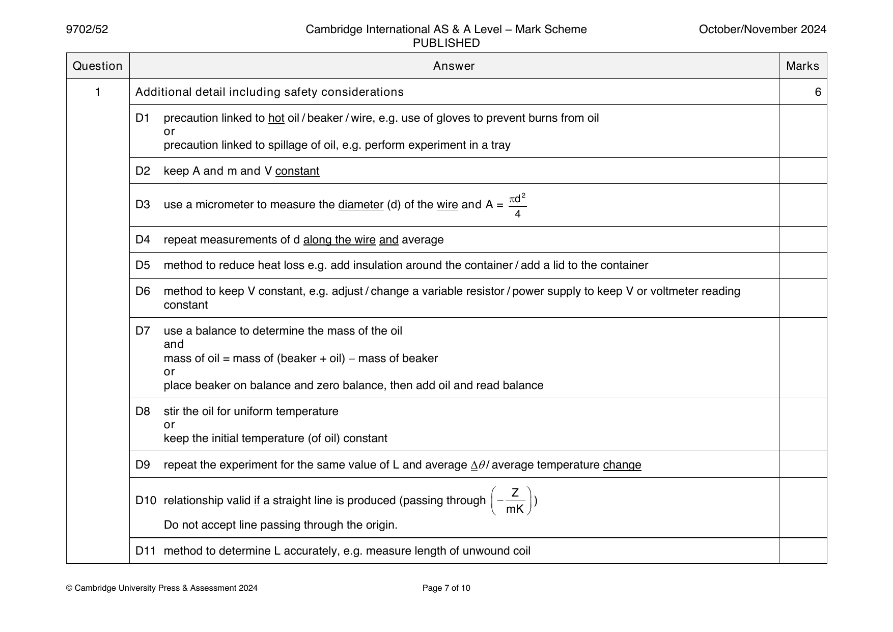
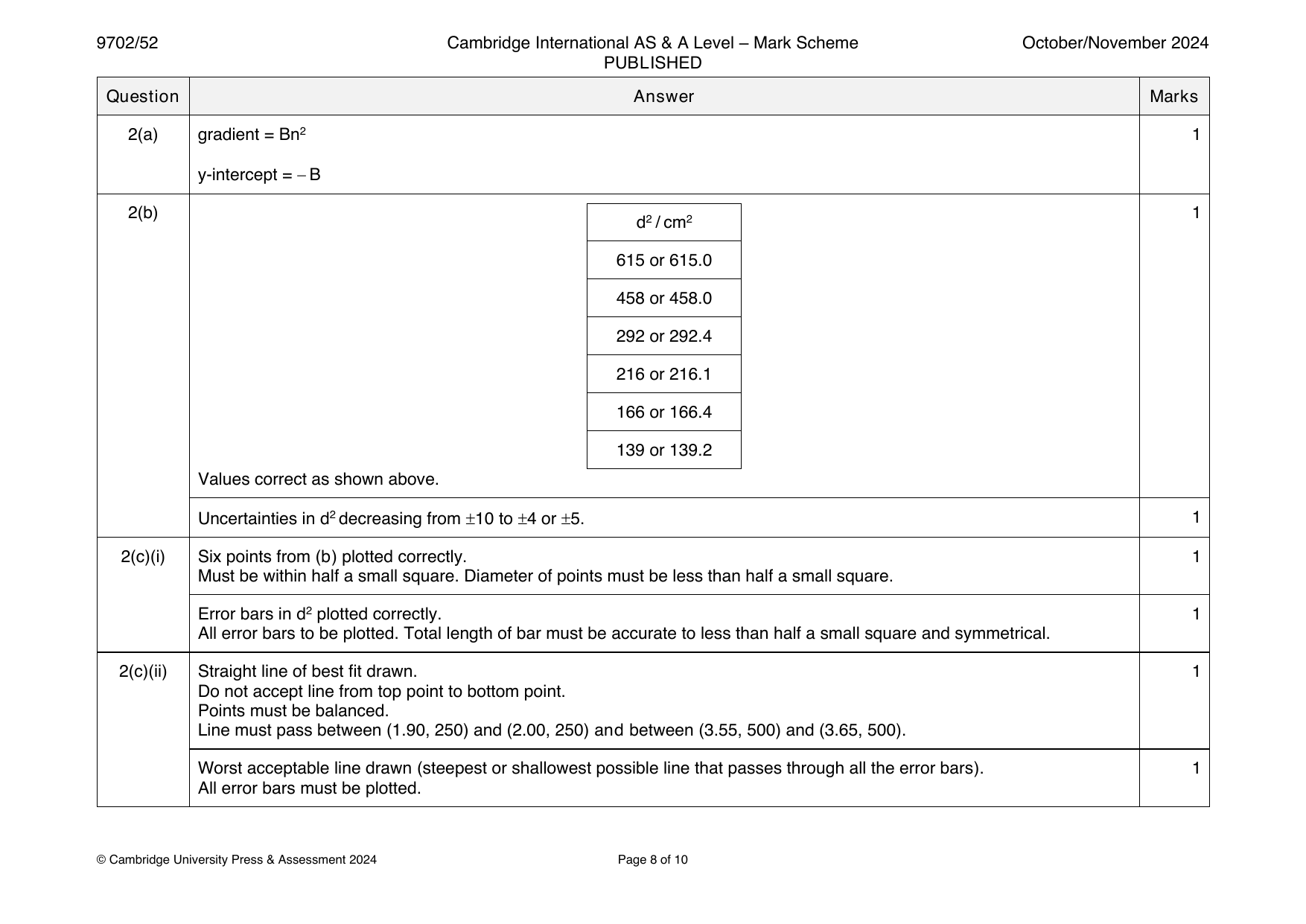
9702-2021-m-52-q01
March 2021 · Paper 52 · Question 1 · 15 marks
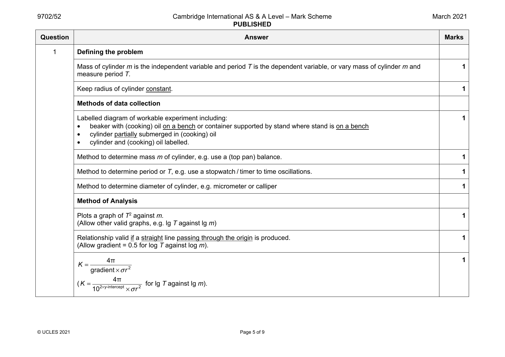
1 Defining the problem
Mass of cylinder m is the independent variable and period T is the dependent variable, or vary mass of cylinder m and 1
measure period T.
Keep radius of cylinder constant. 1
Methods of data collection
Labelled diagram of workable experiment including: 1
• beaker with (cooking) oil on a bench or container supported by stand where stand is on a bench
• cylinder partially submerged in (cooking) oil
• cylinder and (cooking) oil labelled.
Method to determine mass m of cylinder, e.g. use a (top pan) balance. 1
Method to determine period or T, e.g. use a stopwatch / timer to time oscillations. 1
Method to determine diameter of cylinder, e.g. micrometer or calliper 1
Method of Analysis
Plots a graph of T2 against m. 1
(Allow other valid graphs, e.g. lg T against lg m)
Relationship valid if a straight line passing through the origin is produced. 1
(Allow gradient = 0.5 for log T against log m).
4π 1
K =
gradient×σr2
4π
(K = for lg T against lg m).
102×y-intercept ×σr2
© UCLES 2021 Page 5 of 9
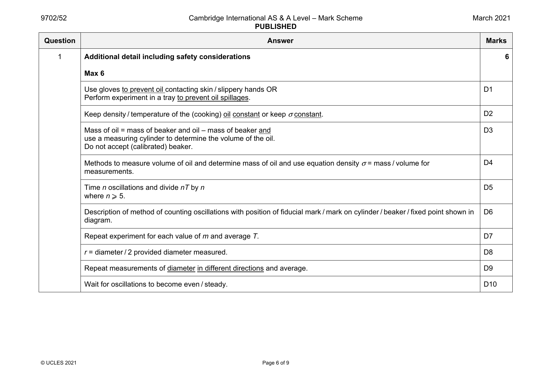
1 Additional detail including safety considerations 6
Max 6
Use gloves to prevent oil contacting skin / slippery hands OR D1
Perform experiment in a tray to prevent oil spillages.
Keep density / temperature of the (cooking) oil constant or keep σ constant. D2
Mass of oil = mass of beaker and oil – mass of beaker and D3
use a measuring cylinder to determine the volume of the oil.
Do not accept (calibrated) beaker.
Methods to measure volume of oil and determine mass of oil and use equation density σ = mass / volume for D4
measurements.
Time n oscillations and divide nT by n D5
where n ⩾ 5.
Description of method of counting oscillations with position of fiducial mark / mark on cylinder / beaker / fixed point shown in D6
diagram.
Repeat experiment for each value of m and average T. D7
r = diameter / 2 provided diameter measured. D8
Repeat measurements of diameter in different directions and average. D9
Wait for oscillations to become even / steady. D10
© UCLES 2021 Page 6 of 9
Official mark scheme pages: 5, 6 · source PDF URL
9702-2021-m-52-q02
March 2021 · Paper 52 · Question 2 · 15 marks
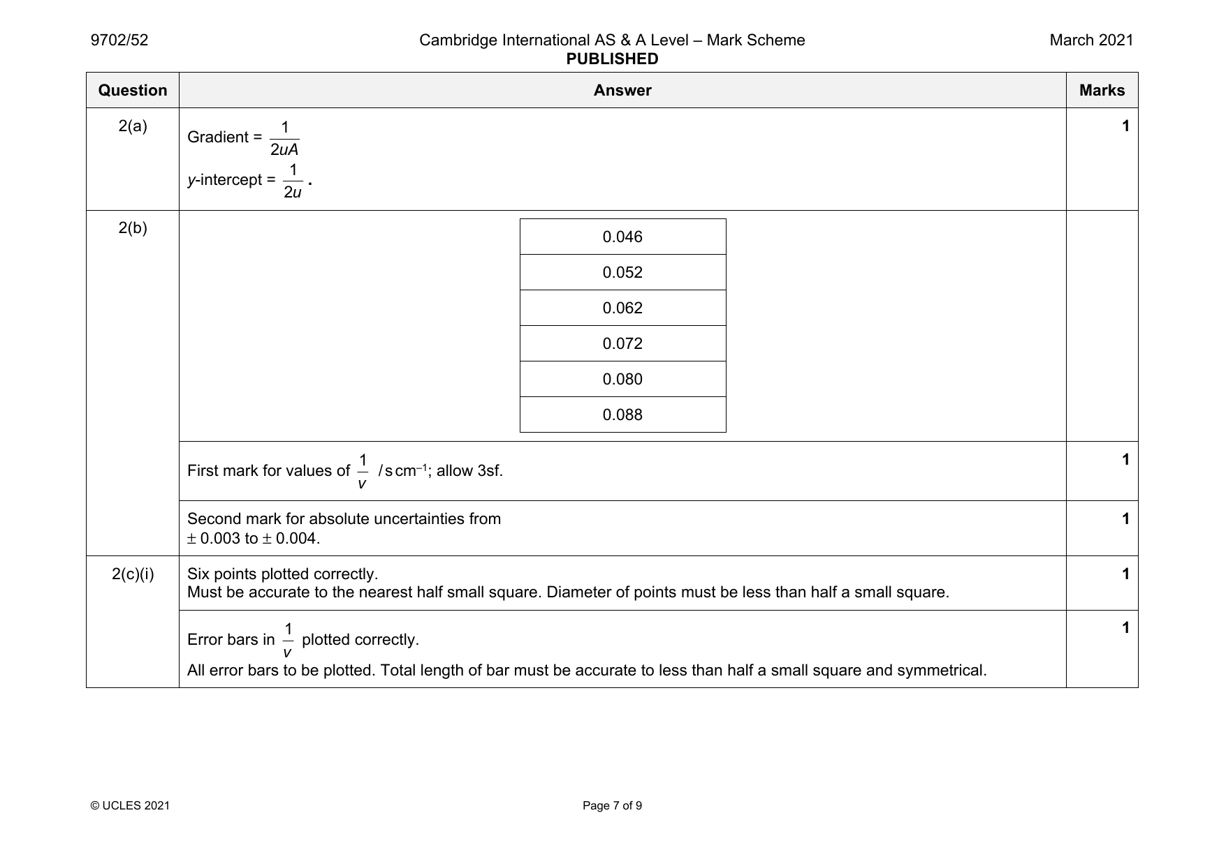
2(a) 1 1
Gradient =
2uA
1
.
y-intercept =
2u
2(b)
0.046
0.052
0.062
0.072
0.080
0.088
1 1
First mark for values of / s cm–1; allow 3sf.
v
Second mark for absolute uncertainties from 1
± 0.003 to ± 0.004.
2(c)(i) Six points plotted correctly. 1
Must be accurate to the nearest half small square. Diameter of points must be less than half a small square.
1 1
Error bars in plotted correctly.
v
All error bars to be plotted. Total length of bar must be accurate to less than half a small square and symmetrical.
© UCLES 2021 Page 7 of 9
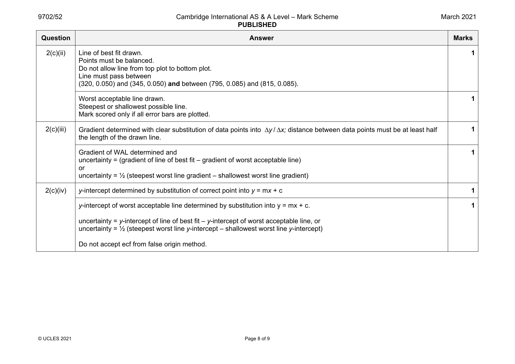
2(c)(ii) Line of best fit drawn. 1
Points must be balanced.
Do not allow line from top plot to bottom plot.
Line must pass between
(320, 0.050) and (345, 0.050) and between (795, 0.085) and (815, 0.085).
Worst acceptable line drawn. 1
Steepest or shallowest possible line.
Mark scored only if all error bars are plotted.
2(c)(iii) Gradient determined with clear substitution of data points into Δy / Δx; distance between data points must be at least half 1
the length of the drawn line.
Gradient of WAL determined and 1
uncertainty = (gradient of line of best fit – gradient of worst acceptable line)
or
uncertainty = ½ (steepest worst line gradient – shallowest worst line gradient)
2(c)(iv) y-intercept determined by substitution of correct point into y = mx + c 1
y-intercept of worst acceptable line determined by substitution into y = mx + c. 1
uncertainty = y-intercept of line of best fit – y-intercept of worst acceptable line, or
uncertainty = ½ (steepest worst line y-intercept – shallowest worst line y-intercept)
Do not accept ecf from false origin method.
© UCLES 2021 Page 8 of 9
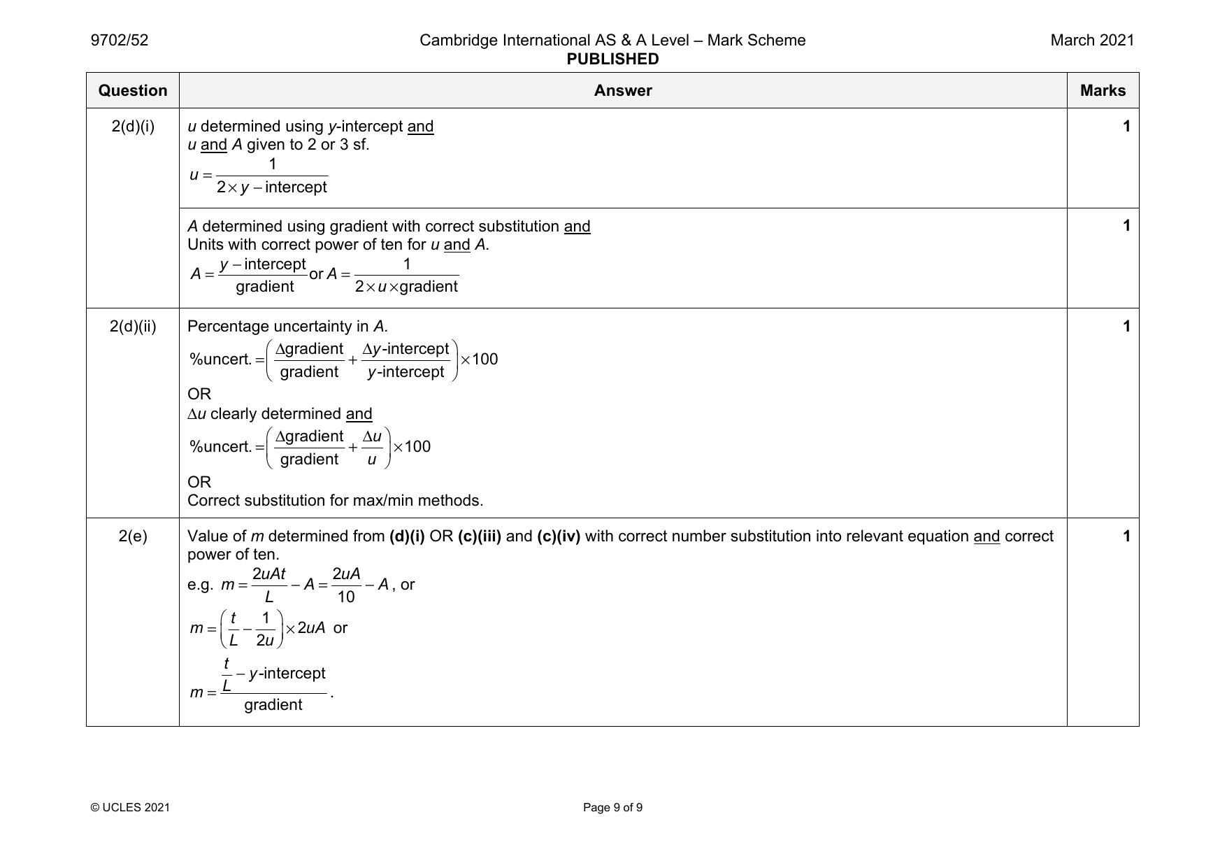
2(d)(i) u determined using y-intercept and 1
u and A given to 2 or 3 sf.
1
u =
2×y −intercept
A determined using gradient with correct substitution and 1
Units with correct power of ten for u and A.
y −intercept 1
A= or A=
gradient 2×u× gradient
2(d)(ii) Percentage uncertainty in A. 1
Δgradient Δy-intercept
%uncert.=
+
×100
gradient y-intercept
OR
Δu clearly determined and
Δgradient Δu
%uncert.=
+
×100
gradient u
OR
Correct substitution for max/min methods.
2(e) Value of m determined from (d)(i) OR (c)(iii) and (c)(iv) with correct number substitution into relevant equation and correct 1
power of ten.
2uAt 2uA
e.g. m= −A= −A, or
L 10
t 1
m= − ×2uA or
L 2u
t
−y-intercept
m= L .
gradient
© UCLES 2021 Page 9 of 9
Official mark scheme pages: 7, 8, 9 · source PDF URL
9702-2021-mj-51-q01
May/June 2021 · Paper 51 · Question 1 · 15 marks
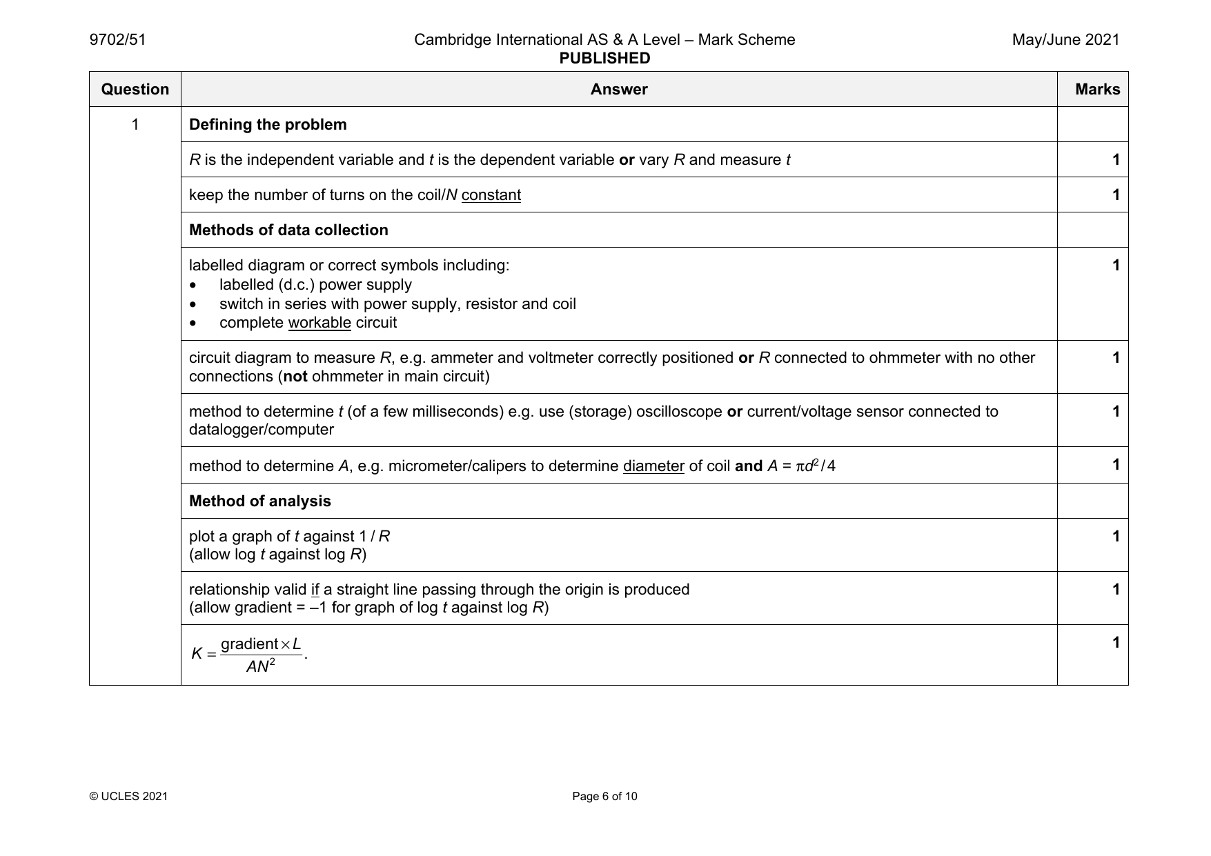
1 Defining the problem
R is the independent variable and t is the dependent variable or vary R and measure t 1
keep the number of turns on the coil/N constant 1
Methods of data collection
labelled diagram or correct symbols including: 1
• labelled (d.c.) power supply
• switch in series with power supply, resistor and coil
• complete workable circuit
circuit diagram to measure R, e.g. ammeter and voltmeter correctly positioned or R connected to ohmmeter with no other 1
connections (not ohmmeter in main circuit)
method to determine t (of a few milliseconds) e.g. use (storage) oscilloscope or current/voltage sensor connected to 1
datalogger/computer
method to determine A, e.g. micrometer/calipers to determine diameter of coil and A = πd2/4 1
Method of analysis
plot a graph of t against 1 / R 1
(allow log t against log R)
relationship valid if a straight line passing through the origin is produced 1
(allow gradient = –1 for graph of log t against log R)
gradient×L 1
K = .
AN2
© UCLES 2021 Page 6 of 10
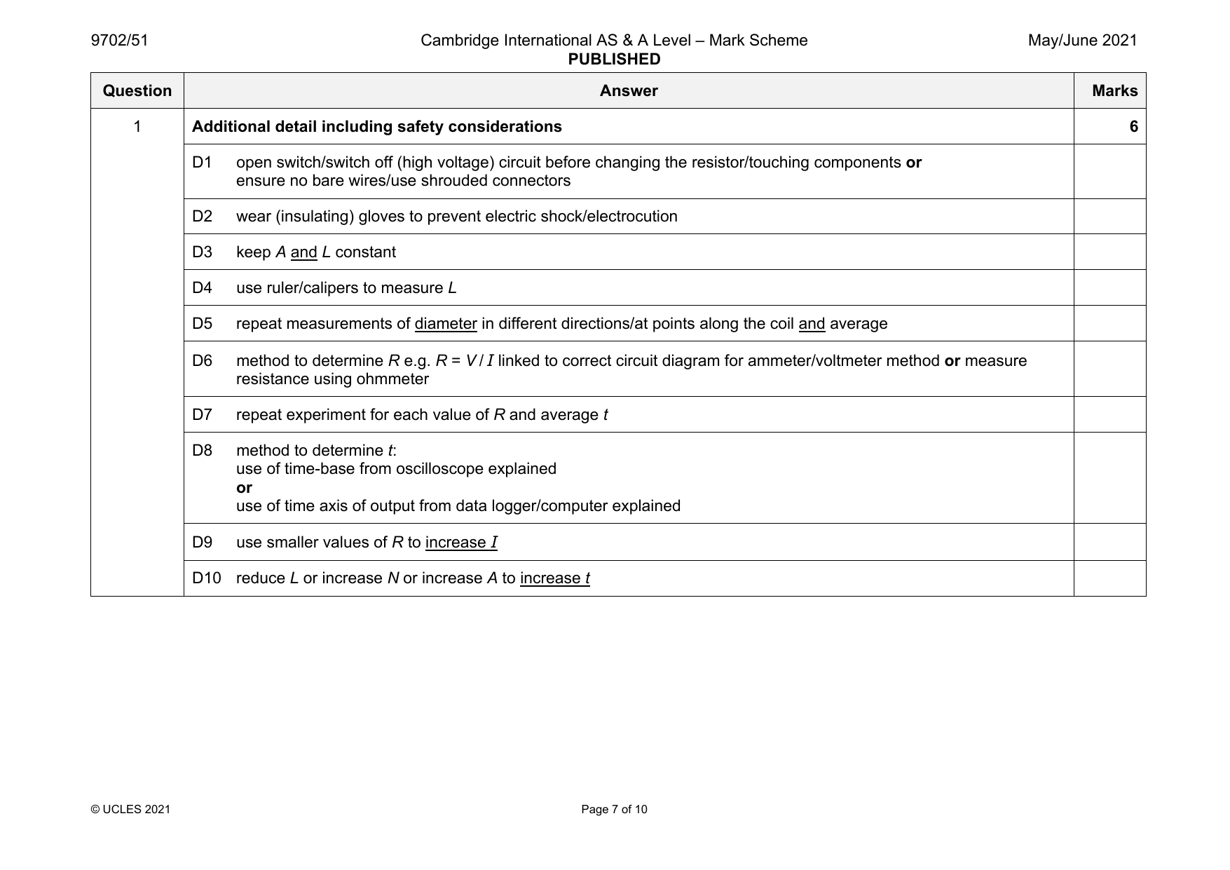
1 Additional detail including safety considerations 6
D1 open switch/switch off (high voltage) circuit before changing the resistor/touching components or
ensure no bare wires/use shrouded connectors
D2 wear (insulating) gloves to prevent electric shock/electrocution
D3 keep A and L constant
D4 use ruler/calipers to measure L
D5 repeat measurements of diameter in different directions/at points along the coil and average
D6 method to determine R e.g. R = V / I linked to correct circuit diagram for ammeter/voltmeter method or measure
resistance using ohmmeter
D7 repeat experiment for each value of R and average t
D8 method to determine t:
use of time-base from oscilloscope explained
or
use of time axis of output from data logger/computer explained
D9 use smaller values of R to increase I
D10 reduce L or increase N or increase A to increase t
© UCLES 2021 Page 7 of 10
Official mark scheme pages: 6, 7 · source PDF URL
9702-2021-mj-51-q02
May/June 2021 · Paper 51 · Question 2 · 15 marks
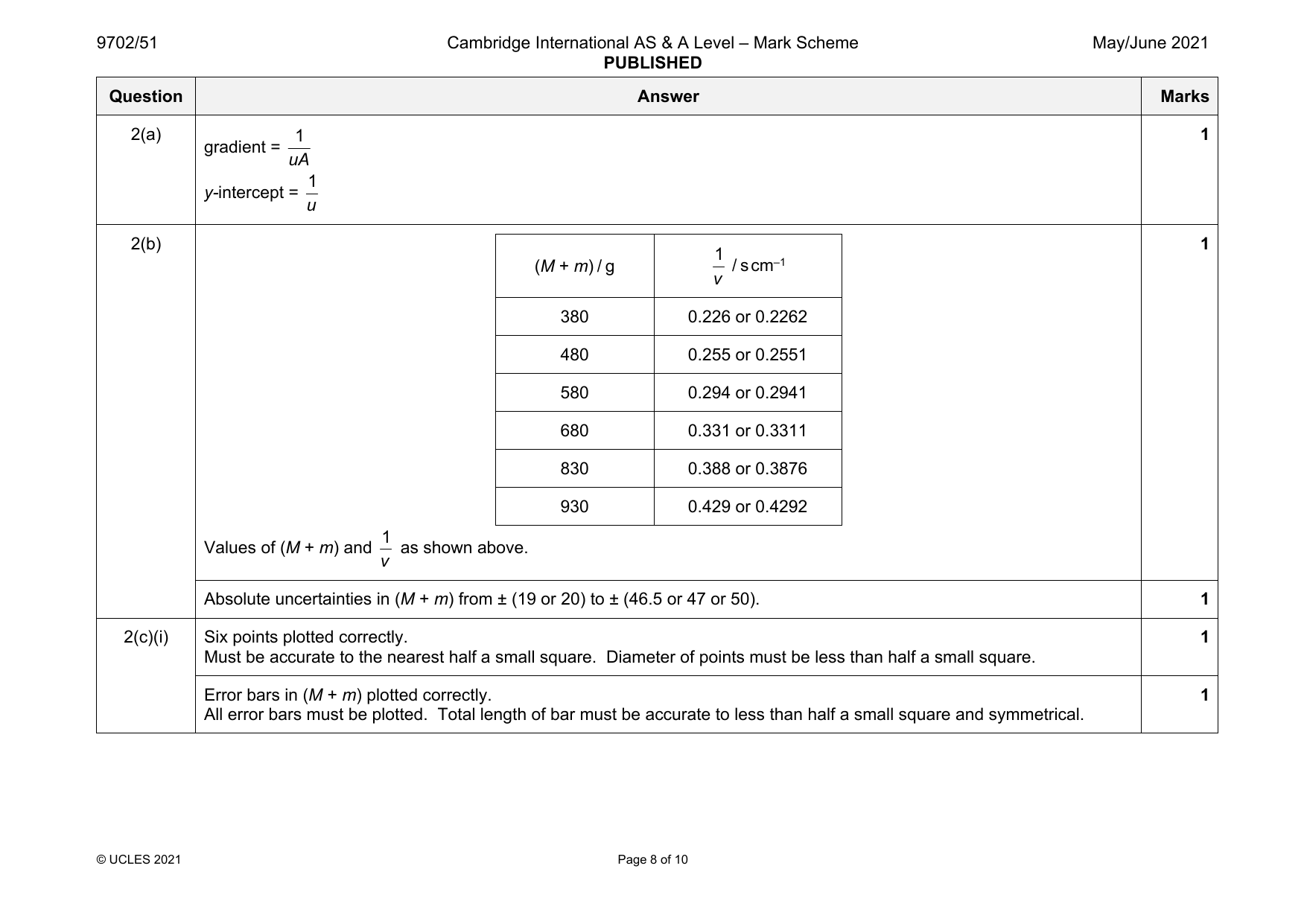
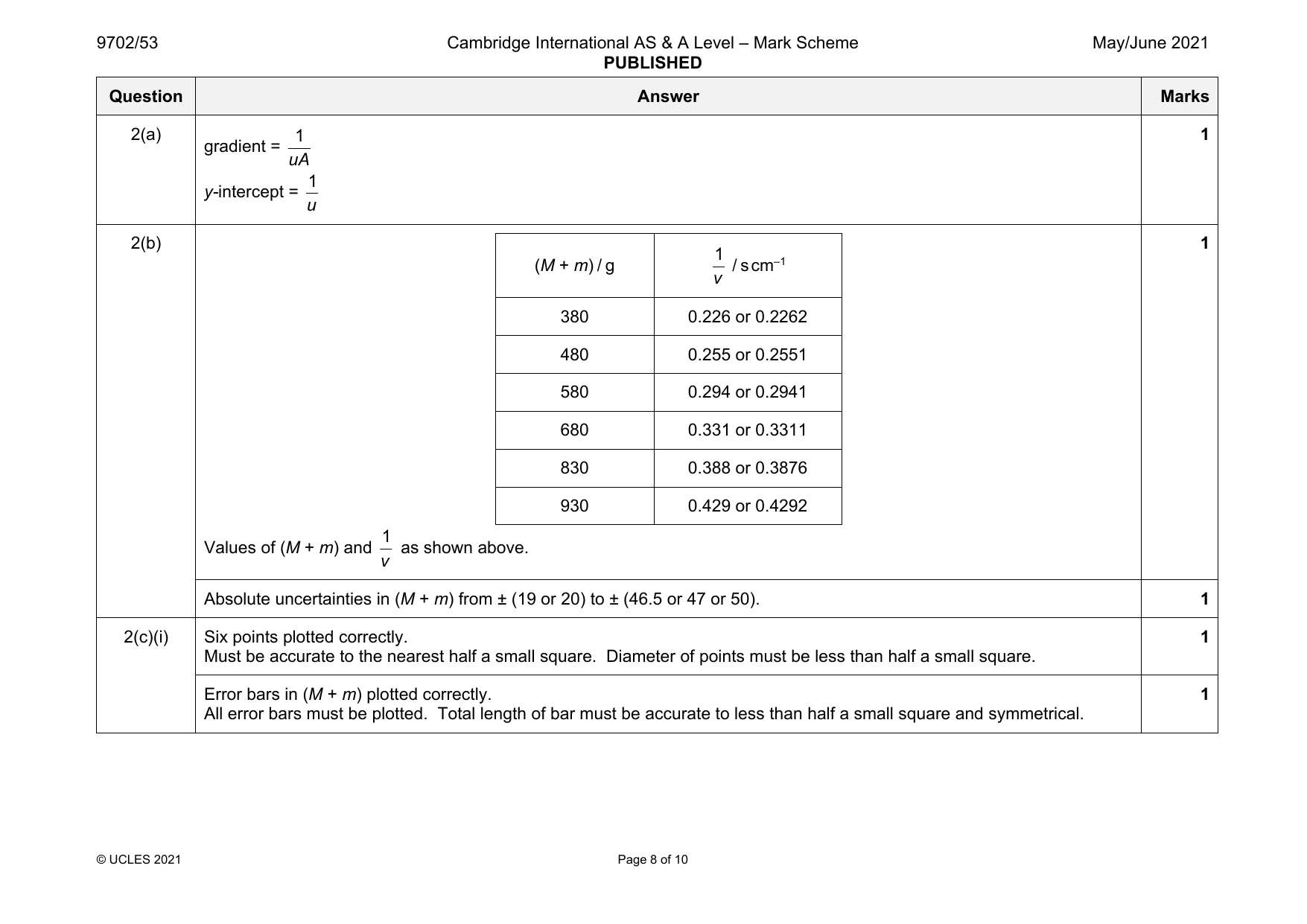
2(a) 1 1
gradient =
uA
1
y-intercept =
u
2(b) 1
1
(M + m) / g / s cm–1
v
380 0.226 or 0.2262
480 0.255 or 0.2551
580 0.294 or 0.2941
680 0.331 or 0.3311
830 0.388 or 0.3876
930 0.429 or 0.4292
1
Values of (M + m) and as shown above.
v
Absolute uncertainties in (M + m) from ± (19 or 20) to ± (46.5 or 47 or 50). 1
2(c)(i) Six points plotted correctly. 1
Must be accurate to the nearest half a small square. Diameter of points must be less than half a small square.
Error bars in (M + m) plotted correctly. 1
All error bars must be plotted. Total length of bar must be accurate to less than half a small square and symmetrical.
© UCLES 2021 Page 8 of 10
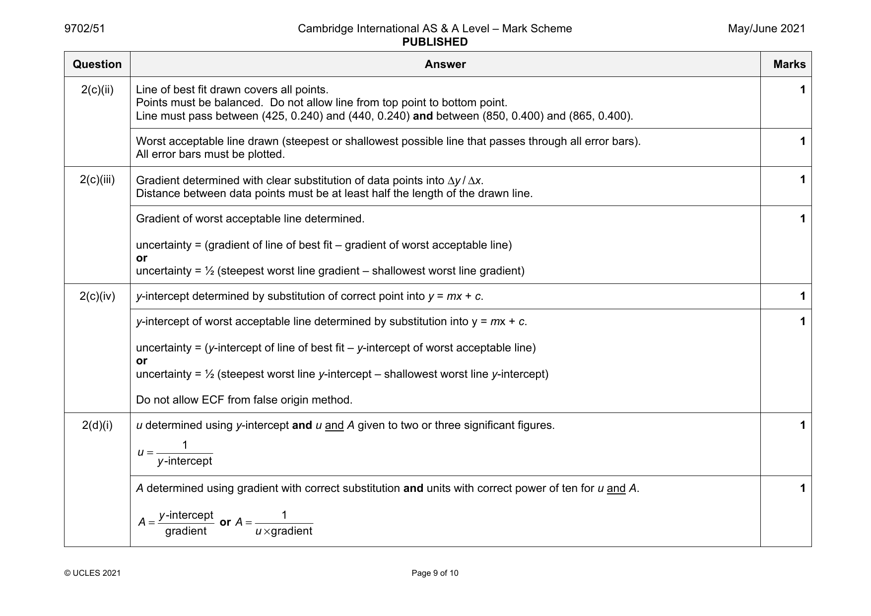
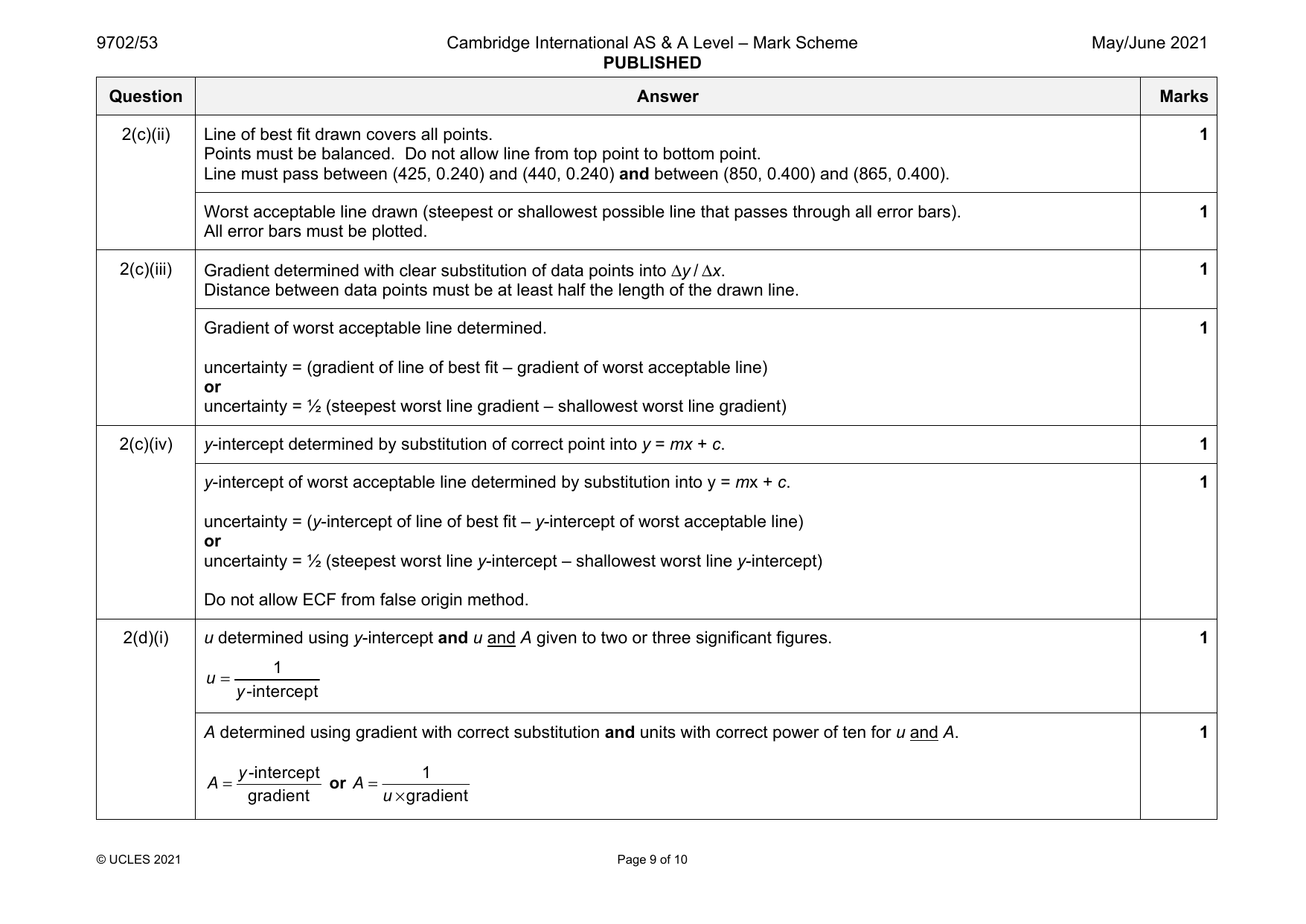
2(c)(ii) Line of best fit drawn covers all points. 1
Points must be balanced. Do not allow line from top point to bottom point.
Line must pass between (425, 0.240) and (440, 0.240) and between (850, 0.400) and (865, 0.400).
Worst acceptable line drawn (steepest or shallowest possible line that passes through all error bars). 1
All error bars must be plotted.
2(c)(iii) Gradient determined with clear substitution of data points into Δy / Δx. 1
Distance between data points must be at least half the length of the drawn line.
Gradient of worst acceptable line determined. 1
uncertainty = (gradient of line of best fit – gradient of worst acceptable line)
or
uncertainty = ½ (steepest worst line gradient – shallowest worst line gradient)
2(c)(iv) y-intercept determined by substitution of correct point into y = mx + c. 1
y-intercept of worst acceptable line determined by substitution into y = mx + c. 1
uncertainty = (y-intercept of line of best fit – y-intercept of worst acceptable line)
or
uncertainty = ½ (steepest worst line y-intercept – shallowest worst line y-intercept)
Do not allow ECF from false origin method.
2(d)(i) u determined using y-intercept and u and A given to two or three significant figures. 1
1
u =
y-intercept
A determined using gradient with correct substitution and units with correct power of ten for u and A. 1
y-intercept 1
A= or A=
gradient u× gradient
© UCLES 2021 Page 9 of 10
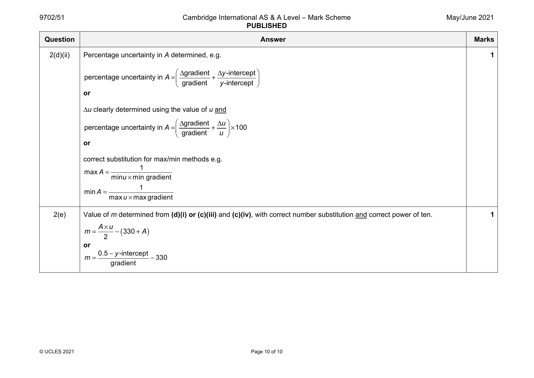
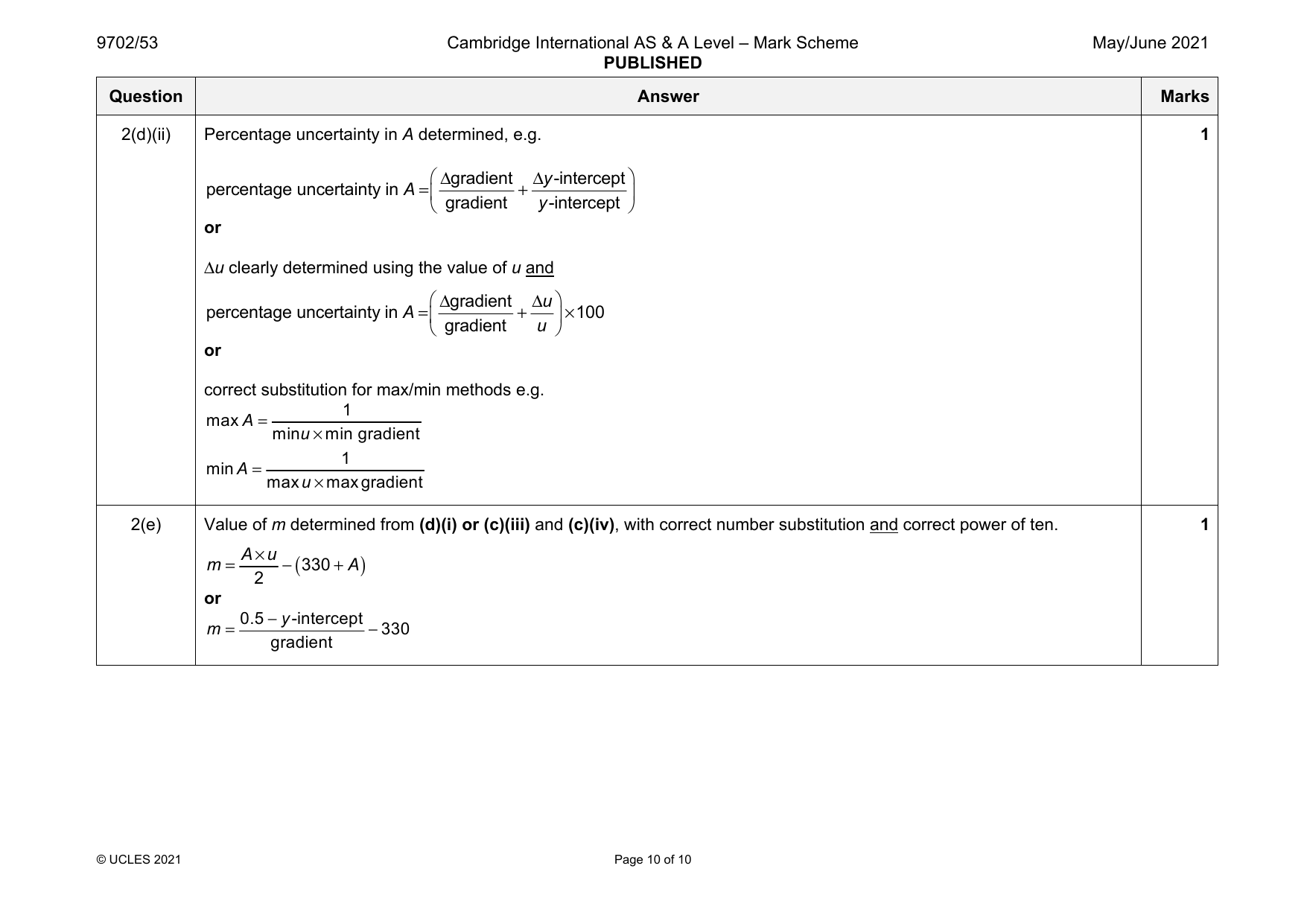
2(d)(ii) Percentage uncertainty in A determined, e.g. 1
Δgradient Δy-intercept
percentage uncertainty in A= +
gradient y-intercept
or
Δu clearly determined using the value of u and
Δgradient Δu
percentage uncertainty in A= + ×100
gradient u
or
correct substitution for max/min methods e.g.
1
maxA=
minu×min gradient
1
minA=
maxu×max gradient
2(e) Value of m determined from (d)(i) or (c)(iii) and (c)(iv), with correct number substitution and correct power of ten. 1
A×u
( )
m= − 330+A
2
or
0.5−y-intercept
m = −330
gradient
© UCLES 2021 Page 10 of 10
Official mark scheme pages: 8, 9, 10 · source PDF URL
9702-2021-mj-52-q01
May/June 2021 · Paper 52 · Question 1 · 15 marks
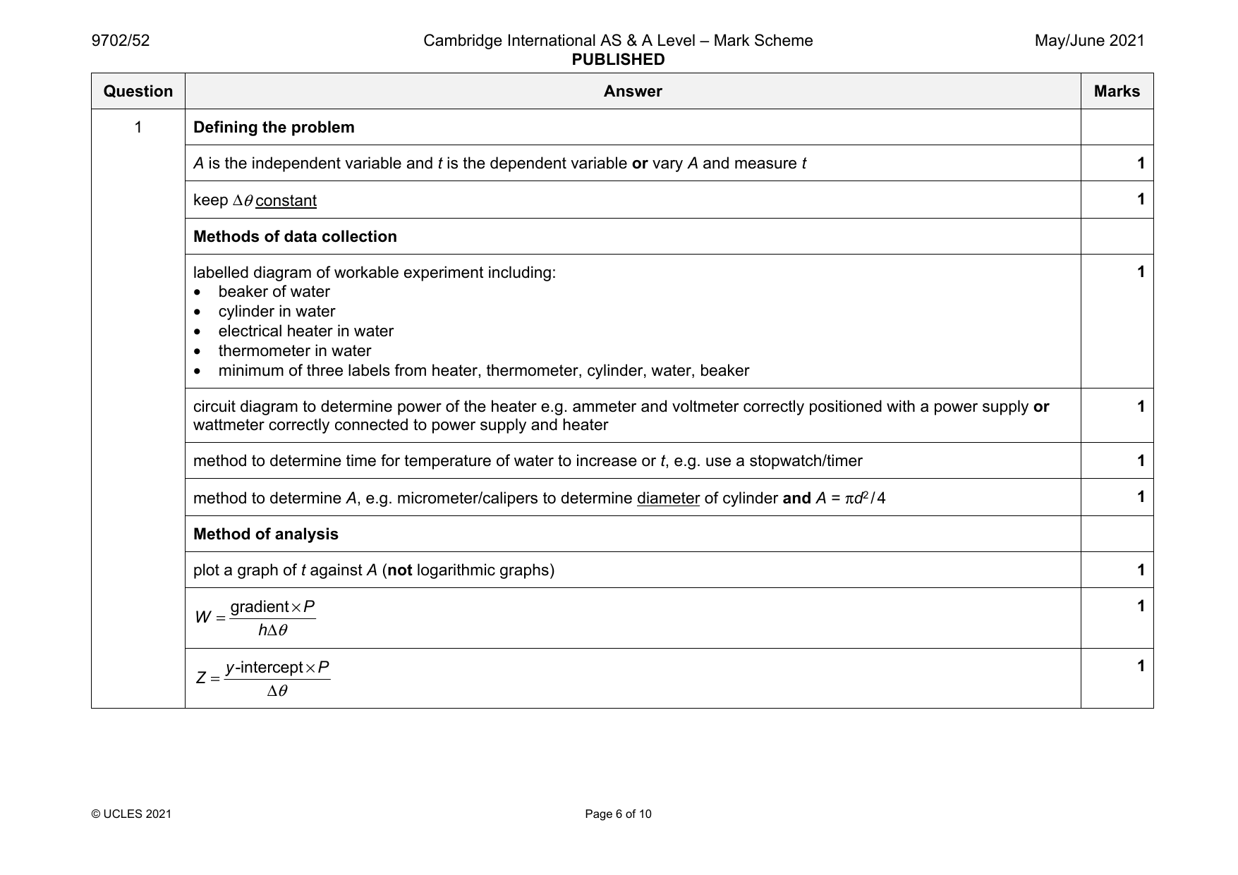
1 Defining the problem
A is the independent variable and t is the dependent variable or vary A and measure t 1
keep Δθ constant 1
Methods of data collection
labelled diagram of workable experiment including: 1
• beaker of water
• cylinder in water
• electrical heater in water
• thermometer in water
• minimum of three labels from heater, thermometer, cylinder, water, beaker
circuit diagram to determine power of the heater e.g. ammeter and voltmeter correctly positioned with a power supply or 1
wattmeter correctly connected to power supply and heater
method to determine time for temperature of water to increase or t, e.g. use a stopwatch/timer 1
method to determine A, e.g. micrometer/calipers to determine diameter of cylinder and A = πd2/4 1
Method of analysis
plot a graph of t against A (not logarithmic graphs) 1
gradient×P 1
W =
hΔθ
y-intercept×P 1
Z =
Δθ
© UCLES 2021 Page 6 of 10
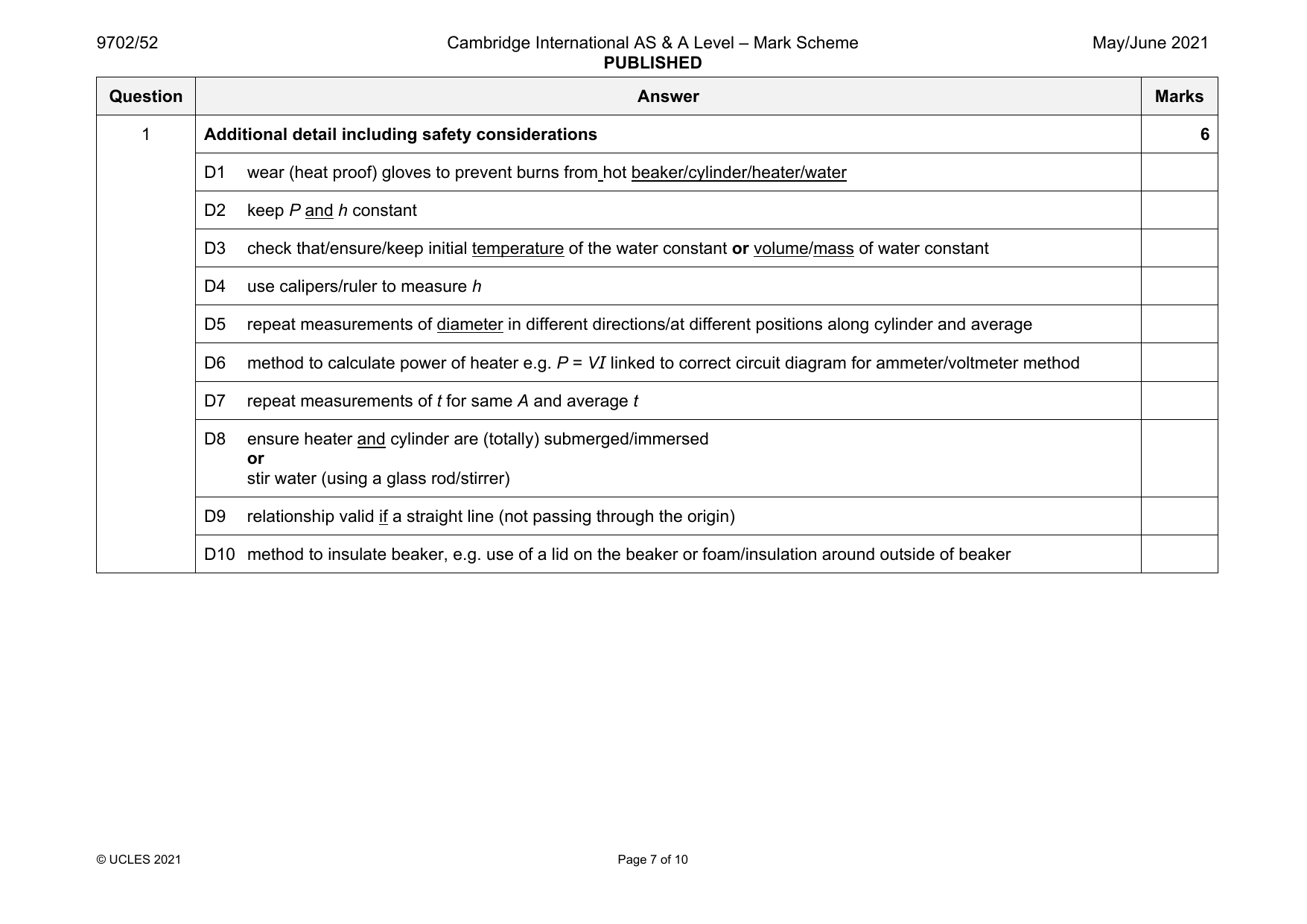
1 Additional detail including safety considerations 6
D1 wear (heat proof) gloves to prevent burns from hot beaker/cylinder/heater/water
D2 keep P and h constant
D3 check that/ensure/keep initial temperature of the water constant or volume/mass of water constant
D4 use calipers/ruler to measure h
D5 repeat measurements of diameter in different directions/at different positions along cylinder and average
D6 method to calculate power of heater e.g. P = VI linked to correct circuit diagram for ammeter/voltmeter method
D7 repeat measurements of t for same A and average t
D8 ensure heater and cylinder are (totally) submerged/immersed
or
stir water (using a glass rod/stirrer)
D9 relationship valid if a straight line (not passing through the origin)
D10 method to insulate beaker, e.g. use of a lid on the beaker or foam/insulation around outside of beaker
© UCLES 2021 Page 7 of 10
Official mark scheme pages: 6, 7 · source PDF URL
9702-2021-mj-52-q02
May/June 2021 · Paper 52 · Question 2 · 15 marks
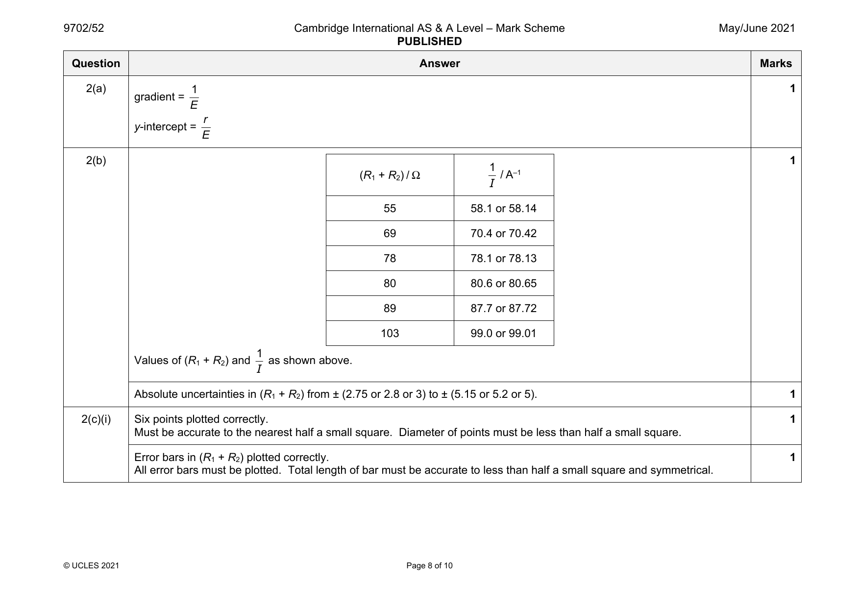
2(a) 1 1
gradient =
E
r
y-intercept =
E
2(b) 1
1
(R + R ) / Ω / A–1
1 2
I
55 58.1 or 58.14
69 70.4 or 70.42
78 78.1 or 78.13
80 80.6 or 80.65
89 87.7 or 87.72
103 99.0 or 99.01
1
Values of (R + R ) and as shown above.
1 2
I
Absolute uncertainties in (R + R ) from ± (2.75 or 2.8 or 3) to ± (5.15 or 5.2 or 5). 1
1 2
2(c)(i) Six points plotted correctly. 1
Must be accurate to the nearest half a small square. Diameter of points must be less than half a small square.
Error bars in (R + R ) plotted correctly. 1
1 2
All error bars must be plotted. Total length of bar must be accurate to less than half a small square and symmetrical.
© UCLES 2021 Page 8 of 10
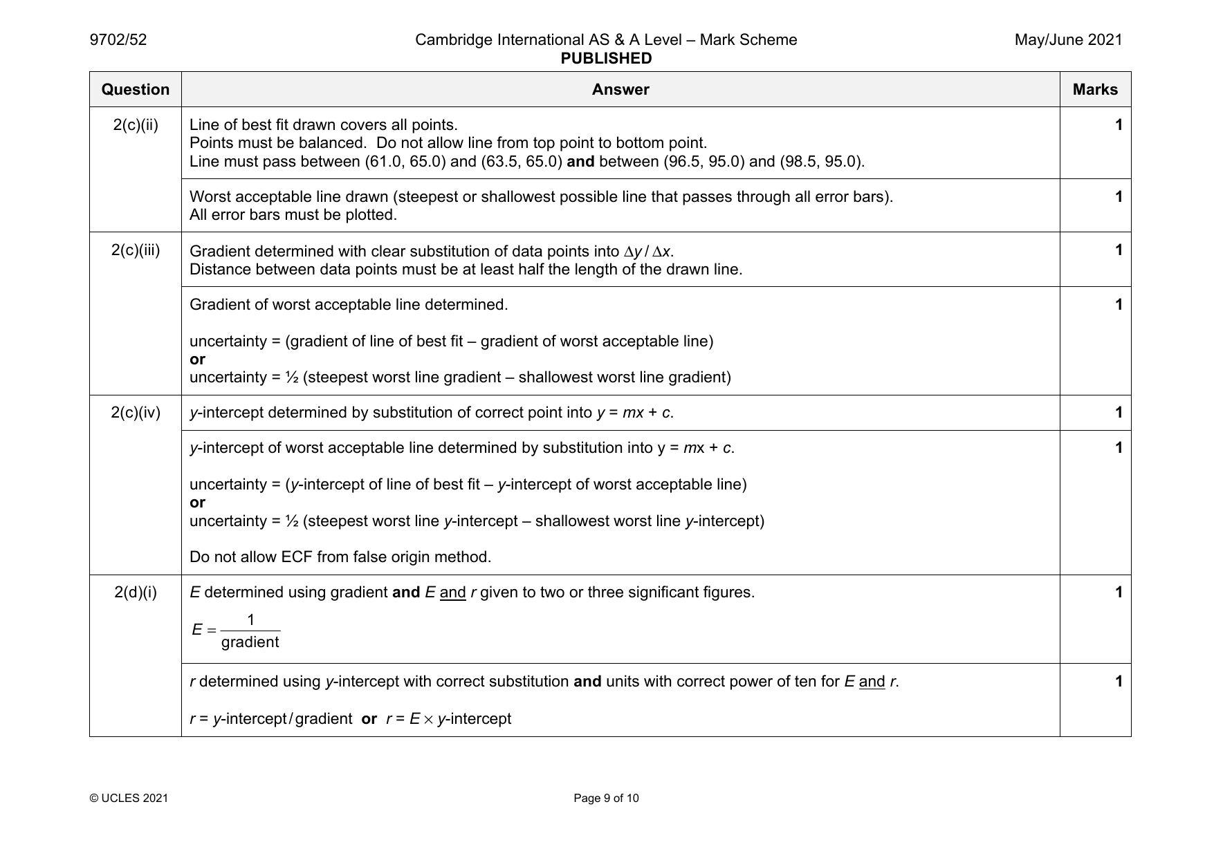
2(c)(ii) Line of best fit drawn covers all points. 1
Points must be balanced. Do not allow line from top point to bottom point.
Line must pass between (61.0, 65.0) and (63.5, 65.0) and between (96.5, 95.0) and (98.5, 95.0).
Worst acceptable line drawn (steepest or shallowest possible line that passes through all error bars). 1
All error bars must be plotted.
2(c)(iii) Gradient determined with clear substitution of data points into Δy / Δx. 1
Distance between data points must be at least half the length of the drawn line.
Gradient of worst acceptable line determined. 1
uncertainty = (gradient of line of best fit – gradient of worst acceptable line)
or
uncertainty = ½ (steepest worst line gradient – shallowest worst line gradient)
2(c)(iv) y-intercept determined by substitution of correct point into y = mx + c. 1
y-intercept of worst acceptable line determined by substitution into y = mx + c. 1
uncertainty = (y-intercept of line of best fit – y-intercept of worst acceptable line)
or
uncertainty = ½ (steepest worst line y-intercept – shallowest worst line y-intercept)
Do not allow ECF from false origin method.
2(d)(i) E determined using gradient and E and r given to two or three significant figures. 1
1
E =
gradient
r determined using y-intercept with correct substitution and units with correct power of ten for E and r. 1
r = y-intercept/gradient or r = E × y-intercept
© UCLES 2021 Page 9 of 10
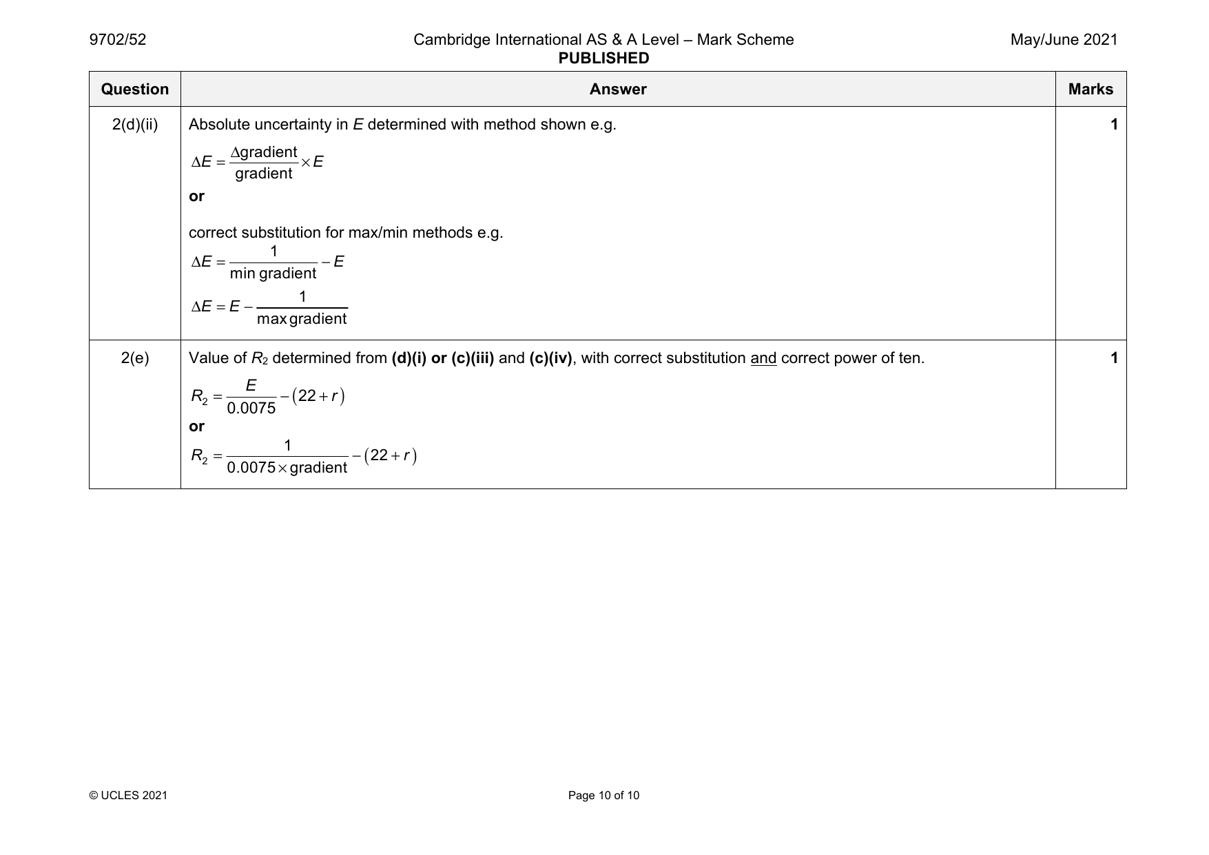
2(d)(ii) Absolute uncertainty in E determined with method shown e.g. 1
Δgradient
ΔE = ×E
gradient
or
correct substitution for max/min methods e.g.
1
ΔE = −E
mingradient
1
ΔE =E −
max gradient
2(e) Value of R determined from (d)(i) or (c)(iii) and (c)(iv), with correct substitution and correct power of ten. 1
2
E ( )
R = − 22+r
2 0.0075
or
R = 1 −( 22+r )
2 0.0075×gradient
© UCLES 2021 Page 10 of 10
Official mark scheme pages: 8, 9, 10 · source PDF URL
9702-2021-mj-53-q01
May/June 2021 · Paper 53 · Question 1 · 15 marks
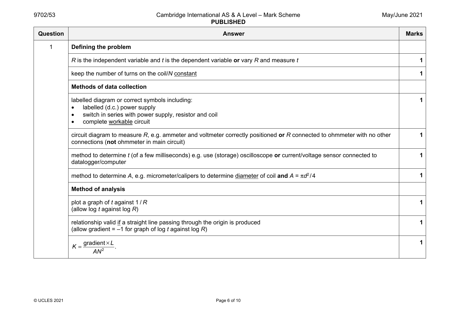
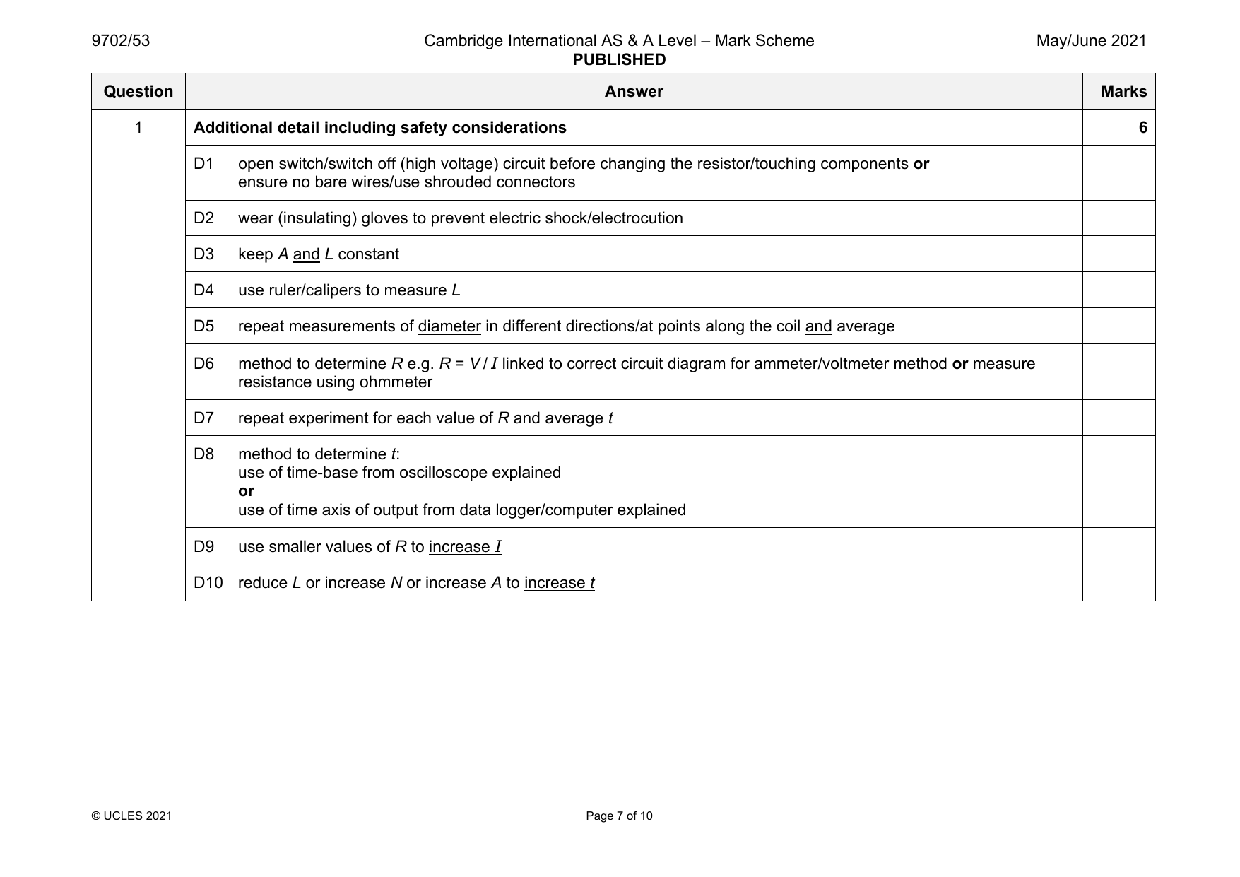
1 Defining the problem
R is the independent variable and t is the dependent variable or vary R and measure t 1
keep the number of turns on the coil/N constant 1
Methods of data collection
labelled diagram or correct symbols including: 1
• labelled (d.c.) power supply
• switch in series with power supply, resistor and coil
• complete workable circuit
circuit diagram to measure R, e.g. ammeter and voltmeter correctly positioned or R connected to ohmmeter with no other 1
connections (not ohmmeter in main circuit)
method to determine t (of a few milliseconds) e.g. use (storage) oscilloscope or current/voltage sensor connected to 1
datalogger/computer
method to determine A, e.g. micrometer/calipers to determine diameter of coil and A = πd2/4 1
Method of analysis
plot a graph of t against 1 / R 1
(allow log t against log R)
relationship valid if a straight line passing through the origin is produced 1
(allow gradient = –1 for graph of log t against log R)
gradient×L 1
K = .
AN2
© UCLES 2021 Page 6 of 10
1 Additional detail including safety considerations 6
D1 open switch/switch off (high voltage) circuit before changing the resistor/touching components or
ensure no bare wires/use shrouded connectors
D2 wear (insulating) gloves to prevent electric shock/electrocution
D3 keep A and L constant
D4 use ruler/calipers to measure L
D5 repeat measurements of diameter in different directions/at points along the coil and average
D6 method to determine R e.g. R = V / I linked to correct circuit diagram for ammeter/voltmeter method or measure
resistance using ohmmeter
D7 repeat experiment for each value of R and average t
D8 method to determine t:
use of time-base from oscilloscope explained
or
use of time axis of output from data logger/computer explained
D9 use smaller values of R to increase I
D10 reduce L or increase N or increase A to increase t
© UCLES 2021 Page 7 of 10
Official mark scheme pages: 6, 7 · source PDF URL
9702-2021-mj-53-q02
May/June 2021 · Paper 53 · Question 2 · 15 marks
2(a) 1 1
gradient =
uA
1
y-intercept =
u
2(b) 1
1
(M + m) / g / s cm–1
v
380 0.226 or 0.2262
480 0.255 or 0.2551
580 0.294 or 0.2941
680 0.331 or 0.3311
830 0.388 or 0.3876
930 0.429 or 0.4292
1
Values of (M + m) and as shown above.
v
Absolute uncertainties in (M + m) from ± (19 or 20) to ± (46.5 or 47 or 50). 1
2(c)(i) Six points plotted correctly. 1
Must be accurate to the nearest half a small square. Diameter of points must be less than half a small square.
Error bars in (M + m) plotted correctly. 1
All error bars must be plotted. Total length of bar must be accurate to less than half a small square and symmetrical.
© UCLES 2021 Page 8 of 10
2(c)(ii) Line of best fit drawn covers all points. 1
Points must be balanced. Do not allow line from top point to bottom point.
Line must pass between (425, 0.240) and (440, 0.240) and between (850, 0.400) and (865, 0.400).
Worst acceptable line drawn (steepest or shallowest possible line that passes through all error bars). 1
All error bars must be plotted.
2(c)(iii) Gradient determined with clear substitution of data points into Δy / Δx. 1
Distance between data points must be at least half the length of the drawn line.
Gradient of worst acceptable line determined. 1
uncertainty = (gradient of line of best fit – gradient of worst acceptable line)
or
uncertainty = ½ (steepest worst line gradient – shallowest worst line gradient)
2(c)(iv) y-intercept determined by substitution of correct point into y = mx + c. 1
y-intercept of worst acceptable line determined by substitution into y = mx + c. 1
uncertainty = (y-intercept of line of best fit – y-intercept of worst acceptable line)
or
uncertainty = ½ (steepest worst line y-intercept – shallowest worst line y-intercept)
Do not allow ECF from false origin method.
2(d)(i) u determined using y-intercept and u and A given to two or three significant figures. 1
1
u =
y-intercept
A determined using gradient with correct substitution and units with correct power of ten for u and A. 1
y-intercept 1
A= or A=
gradient u× gradient
© UCLES 2021 Page 9 of 10
2(d)(ii) Percentage uncertainty in A determined, e.g. 1
Δgradient Δy-intercept
percentage uncertainty in A= +
gradient y-intercept
or
Δu clearly determined using the value of u and
Δgradient Δu
percentage uncertainty in A= + ×100
gradient u
or
correct substitution for max/min methods e.g.
1
maxA=
minu×min gradient
1
minA=
maxu×max gradient
2(e) Value of m determined from (d)(i) or (c)(iii) and (c)(iv), with correct number substitution and correct power of ten. 1
A×u
( )
m= − 330+A
2
or
0.5−y-intercept
m = −330
gradient
© UCLES 2021 Page 10 of 10
Official mark scheme pages: 8, 9, 10 · source PDF URL
9702-2021-on-51-q01
Oct/Nov 2021 · Paper 51 · Question 1 · 15 marks
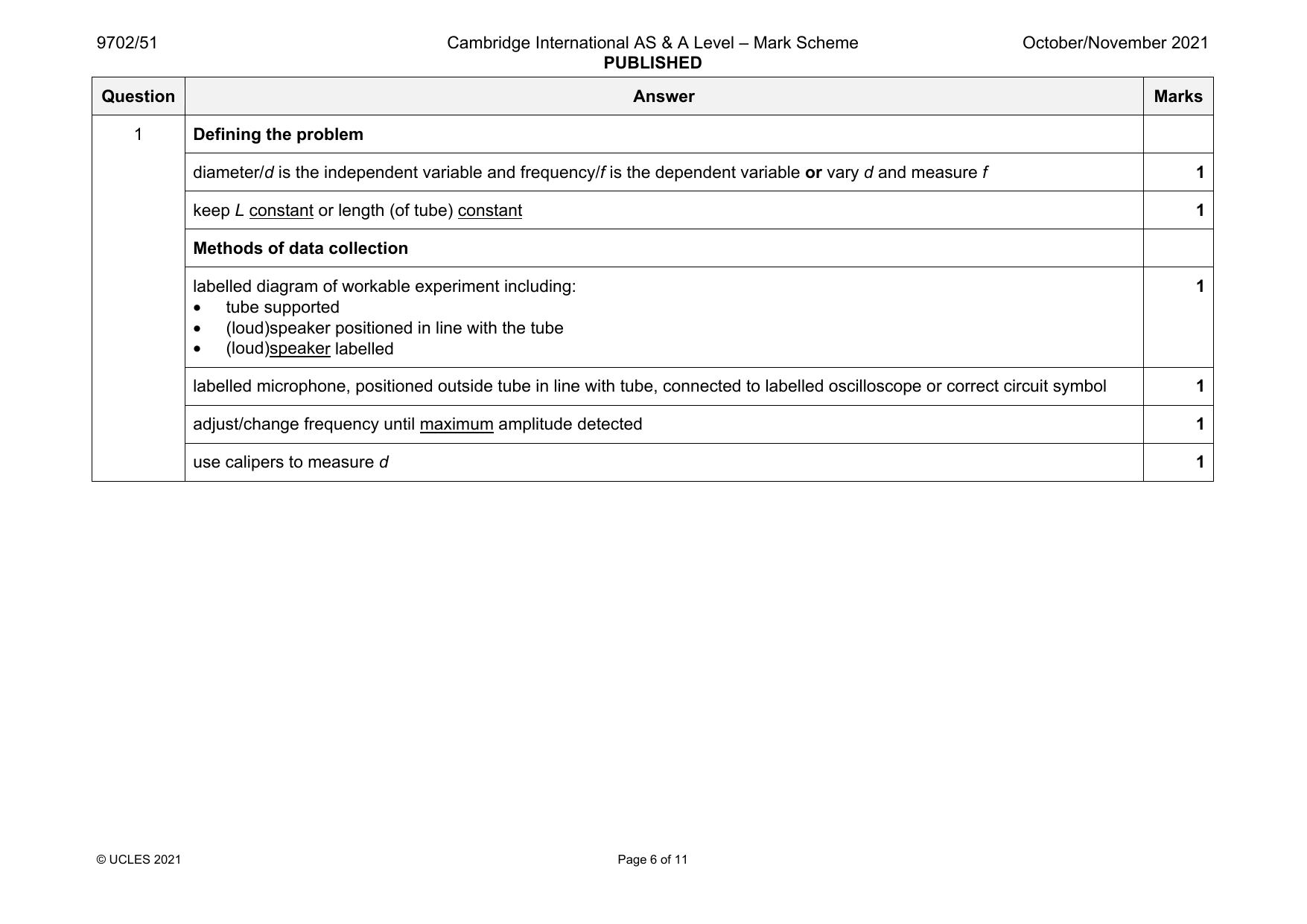
1 Defining the problem
diameter/d is the independent variable and frequency/f is the dependent variable or vary d and measure f 1
keep L constant or length (of tube) constant 1
Methods of data collection
labelled diagram of workable experiment including: 1
• tube supported
• (loud)speaker positioned in line with the tube
• (loud)speaker labelled
labelled microphone, positioned outside tube in line with tube, connected to labelled oscilloscope or correct circuit symbol 1
adjust/change frequency until maximum amplitude detected 1
use calipers to measure d 1
© UCLES 2021 Page 6 of 11
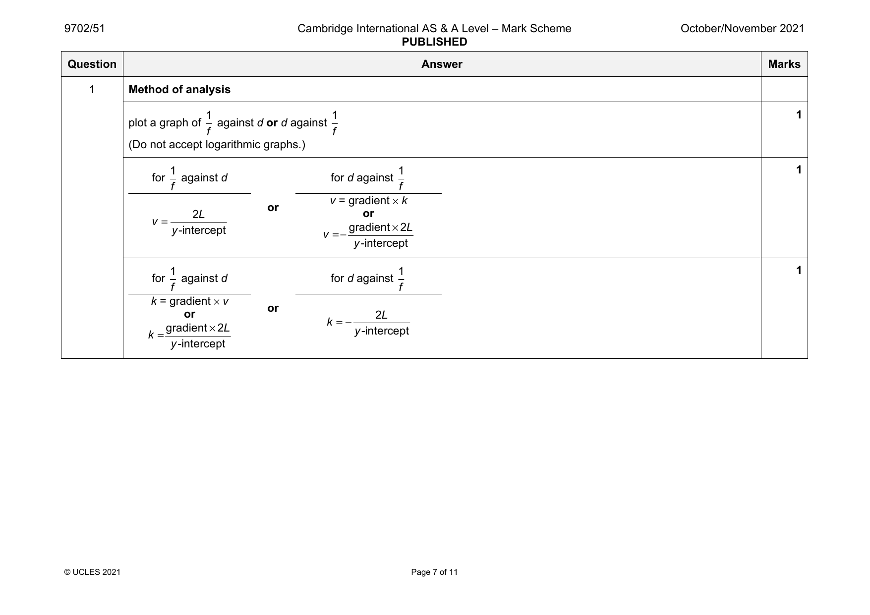
1 Method of analysis
1 1 1
plot a graph of against d or d against
f f
(Do not accept logarithmic graphs.)
1 1 1
for against d for d against
f f
v = gradient × k
or
2L or
v =
y-intercept v = −
gradient×2L
y-intercept
1 1 1
for against d for d against
f f
k = gradient × v
or
or 2L
k =
gradient×2L
k =−
y-intercept
y-intercept
© UCLES 2021 Page 7 of 11
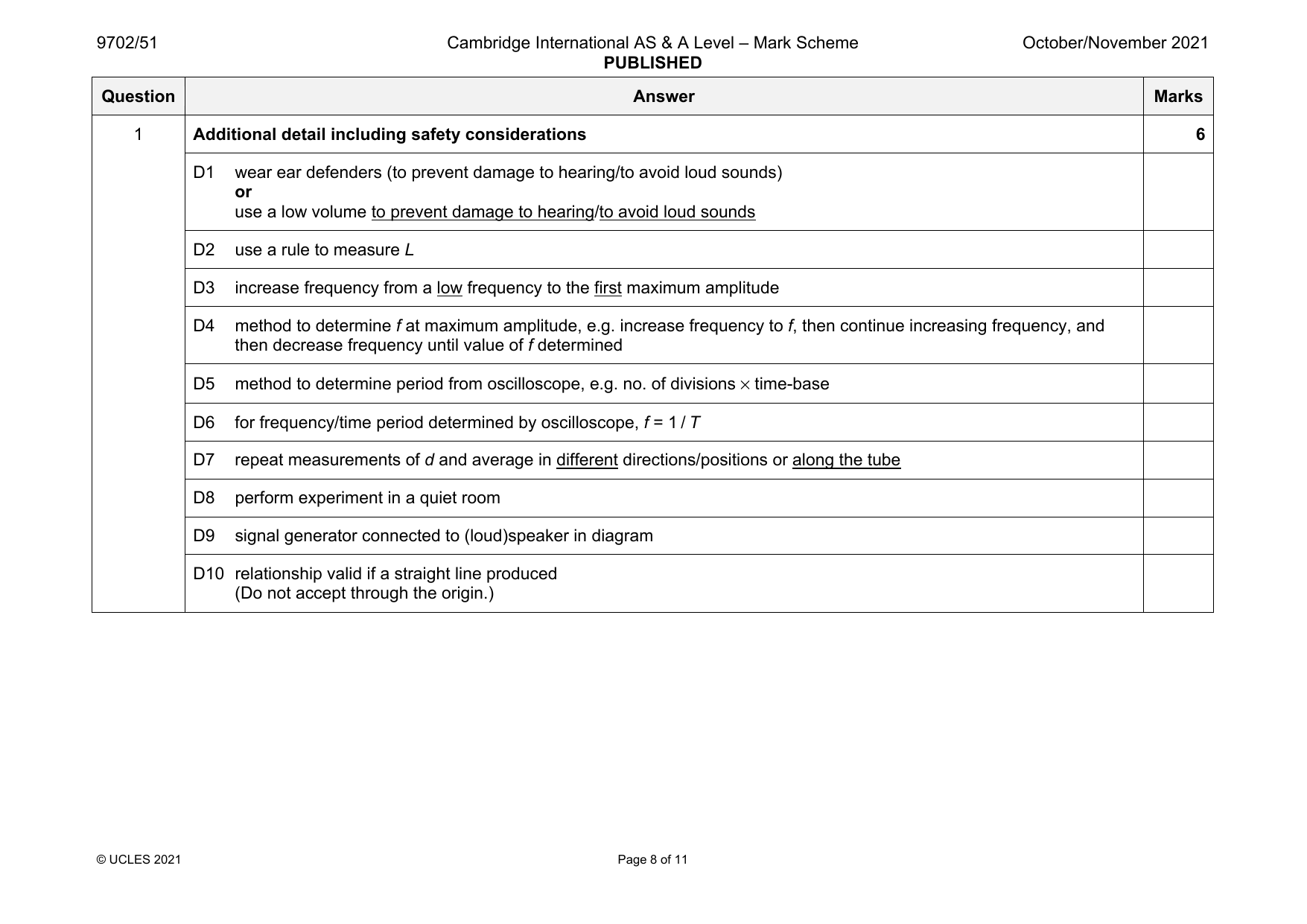
1 Additional detail including safety considerations 6
D1 wear ear defenders (to prevent damage to hearing/to avoid loud sounds)
or
use a low volume to prevent damage to hearing/to avoid loud sounds
D2 use a rule to measure L
D3 increase frequency from a low frequency to the first maximum amplitude
D4 method to determine f at maximum amplitude, e.g. increase frequency to f, then continue increasing frequency, and
then decrease frequency until value of f determined
D5 method to determine period from oscilloscope, e.g. no. of divisions × time-base
D6 for frequency/time period determined by oscilloscope, f = 1 / T
D7 repeat measurements of d and average in different directions/positions or along the tube
D8 perform experiment in a quiet room
D9 signal generator connected to (loud)speaker in diagram
D10 relationship valid if a straight line produced
(Do not accept through the origin.)
© UCLES 2021 Page 8 of 11
Official mark scheme pages: 6, 7, 8 · source PDF URL
9702-2021-on-51-q02
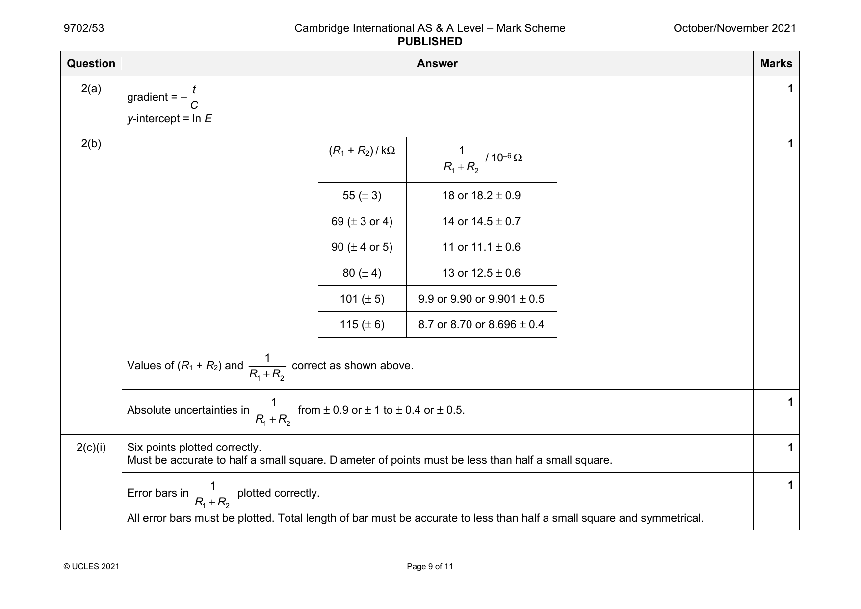
Oct/Nov 2021 · Paper 51 · Question 2 · 15 marks
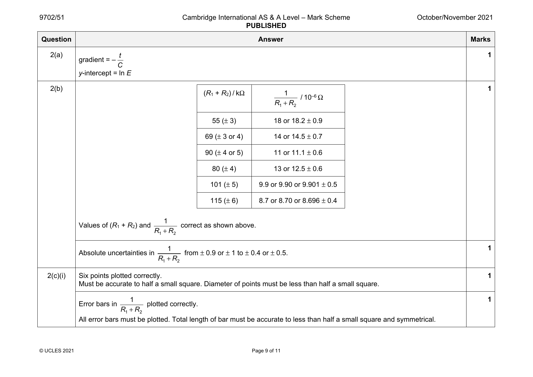
2(a) t 1
gradient = –
C
y-intercept = ln E
2(b) 1
(R + R ) / kΩ 1
1 2 / 10–6 Ω
R +R
1 2
55 (± 3) 18 or 18.2 ± 0.9
69 (± 3 or 4) 14 or 14.5 ± 0.7
90 (± 4 or 5) 11 or 11.1 ± 0.6
80 (± 4) 13 or 12.5 ± 0.6
101 (± 5) 9.9 or 9.90 or 9.901 ± 0.5
115 (± 6) 8.7 or 8.70 or 8.696 ± 0.4
1
Values of (R + R ) and correct as shown above.
1 2 R +R
1 2
1 1
Absolute uncertainties in from ± 0.9 or ± 1 to ± 0.4 or ± 0.5.
R +R
1 2
2(c)(i) Six points plotted correctly. 1
Must be accurate to half a small square. Diameter of points must be less than half a small square.
1 1
Error bars in plotted correctly.
R +R
1 2
All error bars must be plotted. Total length of bar must be accurate to less than half a small square and symmetrical.
© UCLES 2021 Page 9 of 11
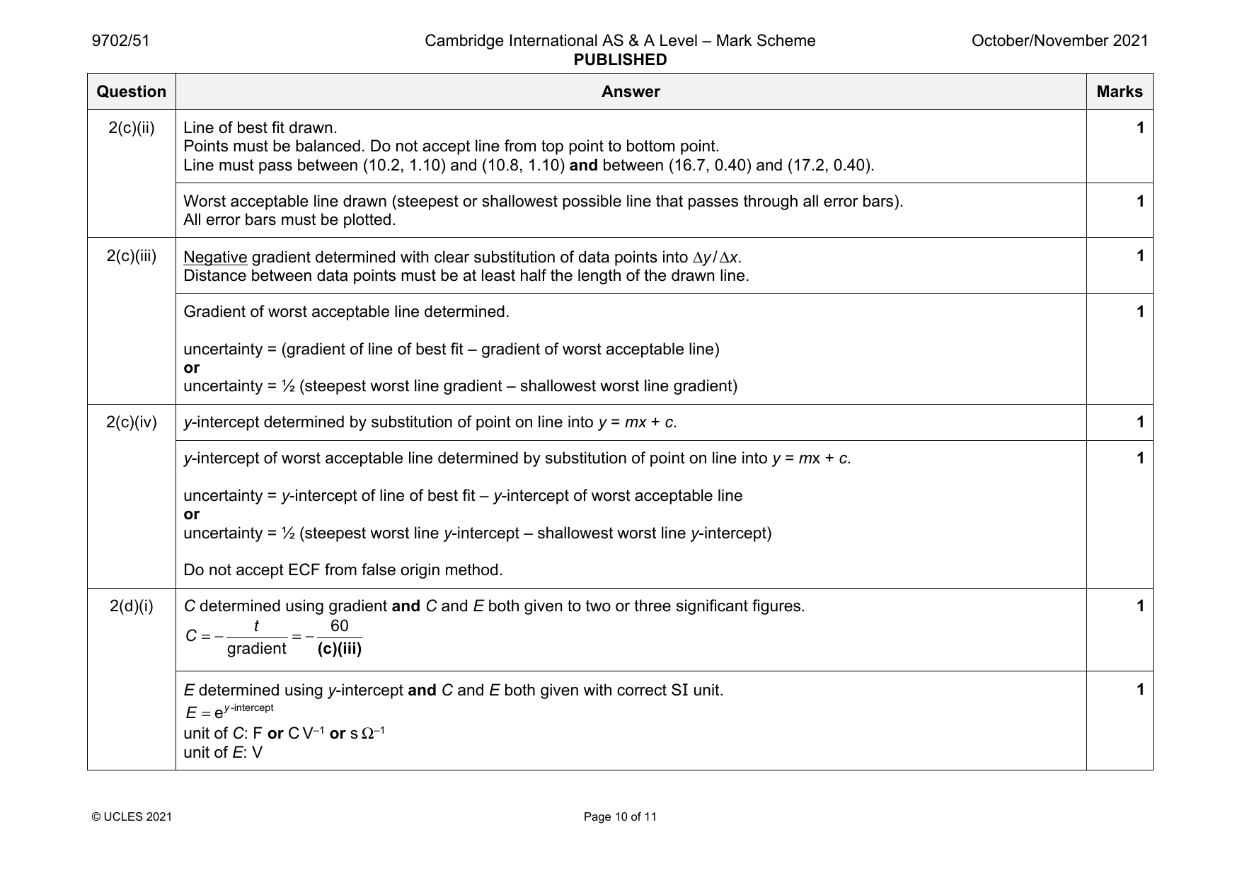
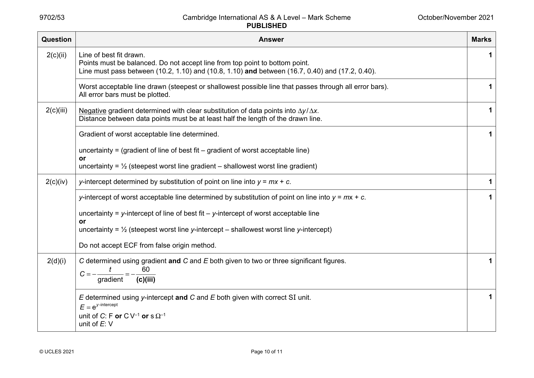
2(c)(ii) Line of best fit drawn. 1
Points must be balanced. Do not accept line from top point to bottom point.
Line must pass between (10.2, 1.10) and (10.8, 1.10) and between (16.7, 0.40) and (17.2, 0.40).
Worst acceptable line drawn (steepest or shallowest possible line that passes through all error bars). 1
All error bars must be plotted.
2(c)(iii) Negative gradient determined with clear substitution of data points into Δy/Δx. 1
Distance between data points must be at least half the length of the drawn line.
Gradient of worst acceptable line determined. 1
uncertainty = (gradient of line of best fit – gradient of worst acceptable line)
or
uncertainty = ½ (steepest worst line gradient – shallowest worst line gradient)
2(c)(iv) y-intercept determined by substitution of point on line into y = mx + c. 1
y-intercept of worst acceptable line determined by substitution of point on line into y = mx + c. 1
uncertainty = y-intercept of line of best fit – y-intercept of worst acceptable line
or
uncertainty = ½ (steepest worst line y-intercept – shallowest worst line y-intercept)
Do not accept ECF from false origin method.
2(d)(i) C determined using gradient and C and E both given to two or three significant figures. 1
t 60
C =− =−
gradient (c)(iii)
E determined using y-intercept and C and E both given with correct SI unit. 1
E =ey-intercept
unit of C: F or C V–1 or s Ω–1
unit of E: V
© UCLES 2021 Page 10 of 11
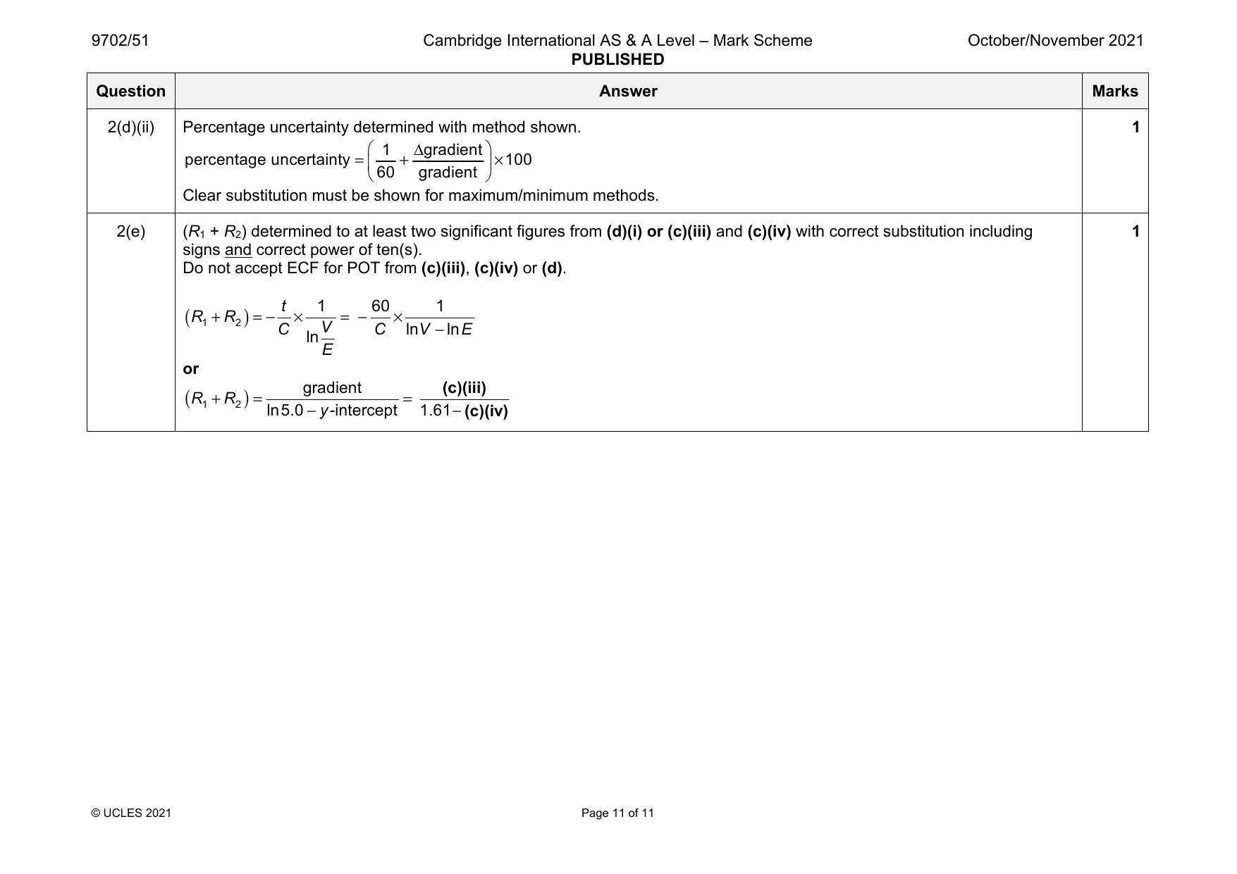
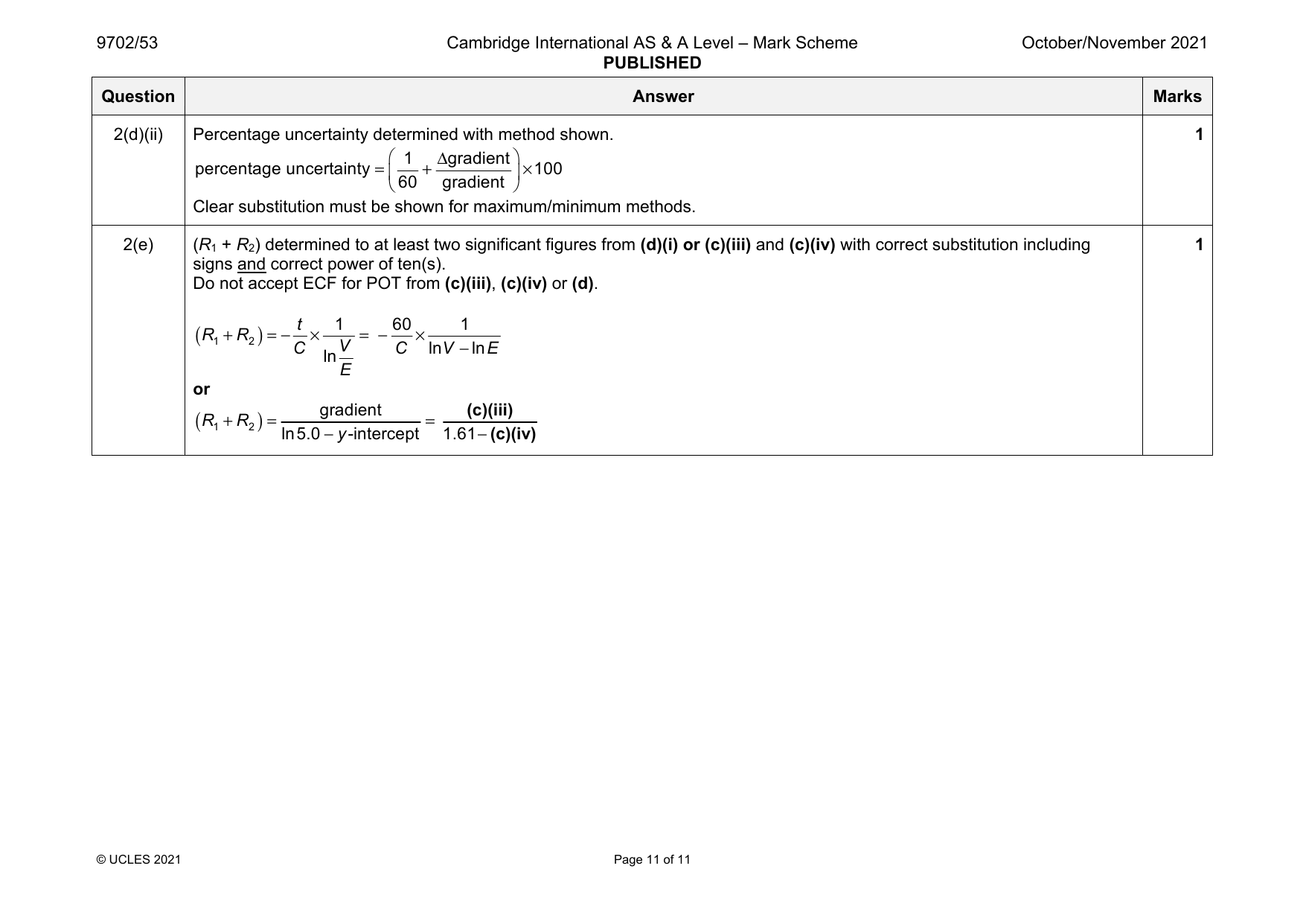
2(d)(ii) Percentage uncertainty determined with method shown. 1
1 Δgradient
percentage uncertainty = + ×100
60 gradient
Clear substitution must be shown for maximum/minimum methods.
2(e) (R + R ) determined to at least two significant figures from (d)(i) or (c)(iii) and (c)(iv) with correct substitution including 1
1 2
signs and correct power of ten(s).
Do not accept ECF for POT from (c)(iii), (c)(iv) or (d).
( R +R )=− t × 1 = − 60 × 1
1 2 C V C lnV −lnE
ln
E
or
( R +R )= gradient = (c)(iii)
1 2 ln5.0−y-intercept 1.61−(c)(iv)
© UCLES 2021 Page 11 of 11
Official mark scheme pages: 9, 10, 11 · source PDF URL
9702-2021-on-52-q01
Oct/Nov 2021 · Paper 52 · Question 1 · 15 marks
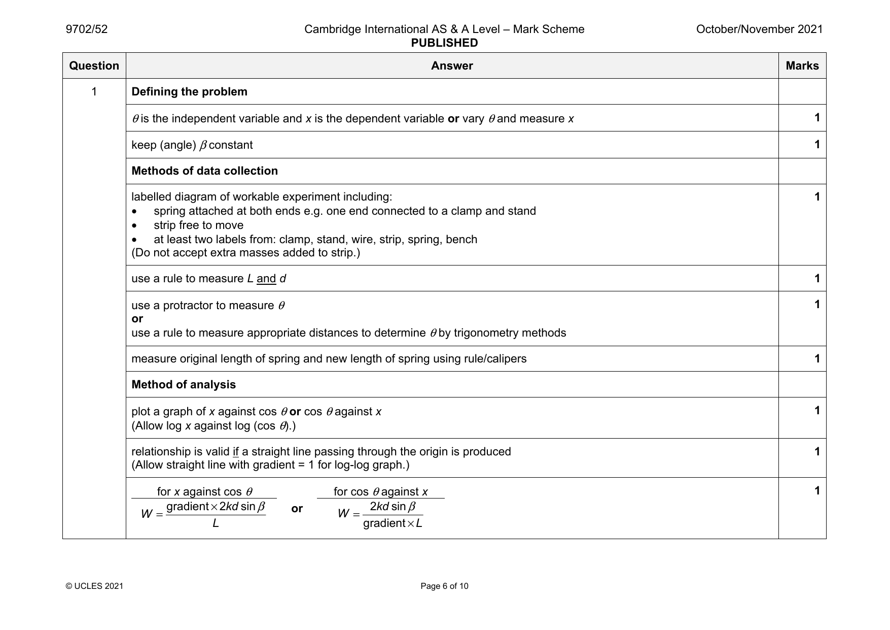
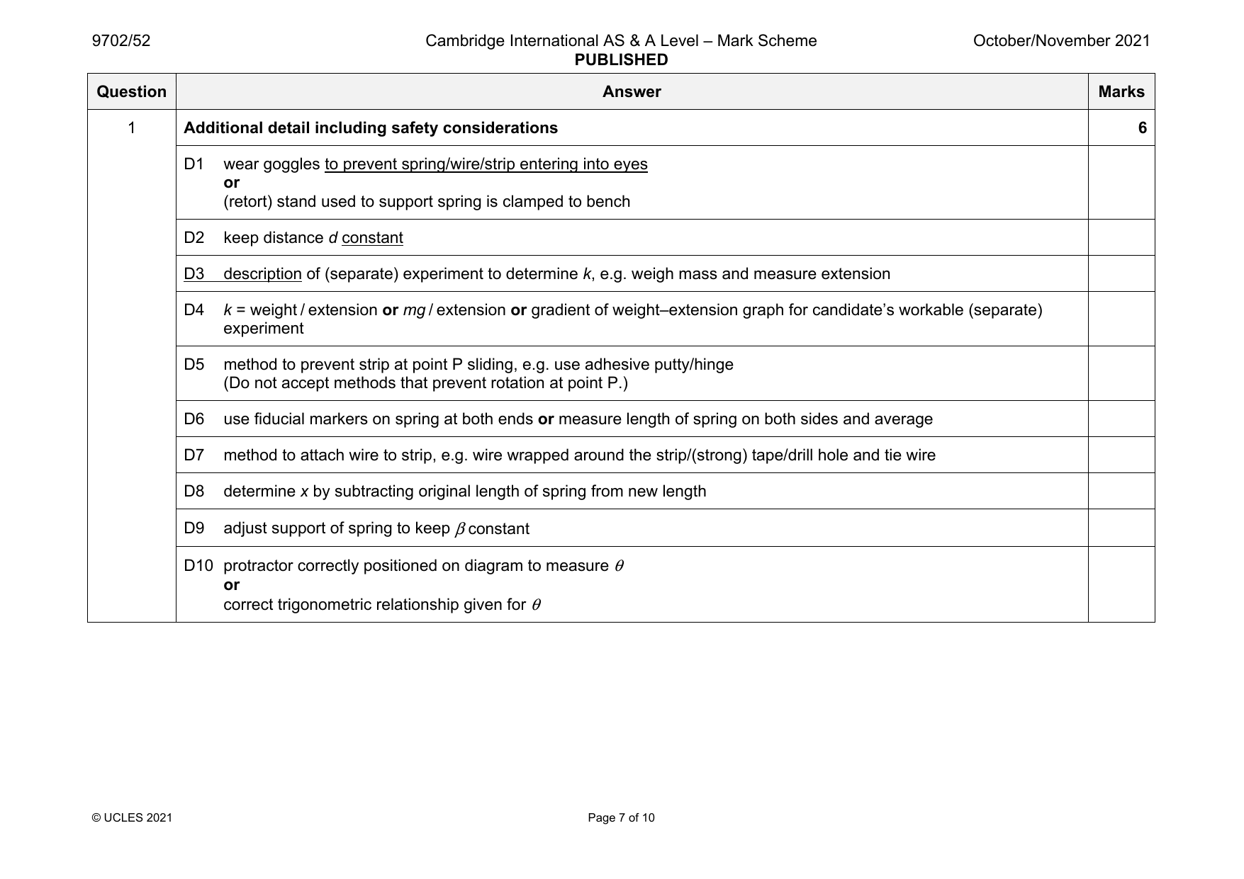
1 Defining the problem
θ is the independent variable and x is the dependent variable or vary θ and measure x 1
keep (angle) β constant 1
Methods of data collection
labelled diagram of workable experiment including: 1
• spring attached at both ends e.g. one end connected to a clamp and stand
• strip free to move
• at least two labels from: clamp, stand, wire, strip, spring, bench
(Do not accept extra masses added to strip.)
use a rule to measure L and d 1
use a protractor to measure θ 1
or
use a rule to measure appropriate distances to determine θ by trigonometry methods
measure original length of spring and new length of spring using rule/calipers 1
Method of analysis
plot a graph of x against cos θ or cos θ against x 1
(Allow log x against log (cos θ).)
relationship is valid if a straight line passing through the origin is produced 1
(Allow straight line with gradient = 1 for log-log graph.)
for x against cos θ for cos θ against x 1
W =
gradient×2kdsinβ
or W =
2kdsinβ
L gradient×L
© UCLES 2021 Page 6 of 10
1 Additional detail including safety considerations 6
D1 wear goggles to prevent spring/wire/strip entering into eyes
or
(retort) stand used to support spring is clamped to bench
D2 keep distance d constant
D3 description of (separate) experiment to determine k, e.g. weigh mass and measure extension
D4 k = weight / extension or mg / extension or gradient of weight–extension graph for candidate’s workable (separate)
experiment
D5 method to prevent strip at point P sliding, e.g. use adhesive putty/hinge
(Do not accept methods that prevent rotation at point P.)
D6 use fiducial markers on spring at both ends or measure length of spring on both sides and average
D7 method to attach wire to strip, e.g. wire wrapped around the strip/(strong) tape/drill hole and tie wire
D8 determine x by subtracting original length of spring from new length
D9 adjust support of spring to keep β constant
D10 protractor correctly positioned on diagram to measure θ
or
correct trigonometric relationship given for θ
© UCLES 2021 Page 7 of 10
Official mark scheme pages: 6, 7 · source PDF URL
9702-2021-on-52-q02
Oct/Nov 2021 · Paper 52 · Question 2 · 15 marks
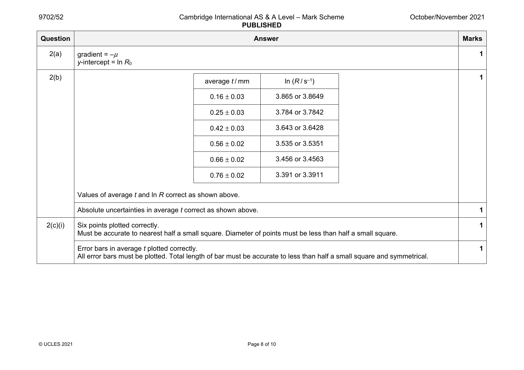
2(a) gradient = –μ 1
y-intercept = ln R
0
2(b) 1
average t / mm ln (R / s–1)
0.16 ± 0.03 3.865 or 3.8649
0.25 ± 0.03 3.784 or 3.7842
0.42 ± 0.03 3.643 or 3.6428
0.56 ± 0.02 3.535 or 3.5351
0.66 ± 0.02 3.456 or 3.4563
0.76 ± 0.02 3.391 or 3.3911
Values of average t and ln R correct as shown above.
Absolute uncertainties in average t correct as shown above. 1
2(c)(i) Six points plotted correctly. 1
Must be accurate to nearest half a small square. Diameter of points must be less than half a small square.
Error bars in average t plotted correctly. 1
All error bars must be plotted. Total length of bar must be accurate to less than half a small square and symmetrical.
© UCLES 2021 Page 8 of 10
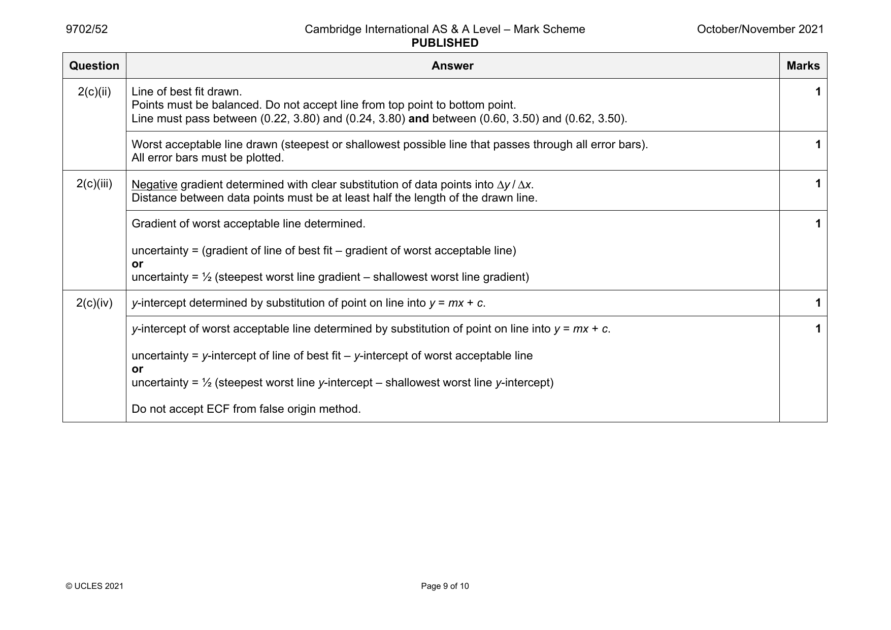
2(c)(ii) Line of best fit drawn. 1
Points must be balanced. Do not accept line from top point to bottom point.
Line must pass between (0.22, 3.80) and (0.24, 3.80) and between (0.60, 3.50) and (0.62, 3.50).
Worst acceptable line drawn (steepest or shallowest possible line that passes through all error bars). 1
All error bars must be plotted.
2(c)(iii) Negative gradient determined with clear substitution of data points into Δy / Δx. 1
Distance between data points must be at least half the length of the drawn line.
Gradient of worst acceptable line determined. 1
uncertainty = (gradient of line of best fit – gradient of worst acceptable line)
or
uncertainty = ½ (steepest worst line gradient – shallowest worst line gradient)
2(c)(iv) y-intercept determined by substitution of point on line into y = mx + c. 1
y-intercept of worst acceptable line determined by substitution of point on line into y = mx + c. 1
uncertainty = y-intercept of line of best fit – y-intercept of worst acceptable line
or
uncertainty = ½ (steepest worst line y-intercept – shallowest worst line y-intercept)
Do not accept ECF from false origin method.
© UCLES 2021 Page 9 of 10
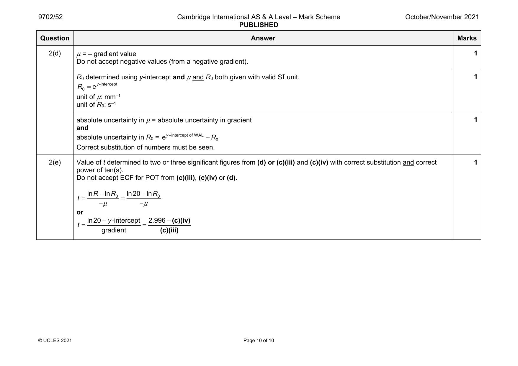
2(d) μ = – gradient value 1
Do not accept negative values (from a negative gradient).
R determined using y-intercept and μ and R both given with valid SI unit. 1
0 0
R =ey-intercept
0
unit of μ: mm–1
unit of R : s–1
0
absolute uncertainty in μ = absolute uncertainty in gradient 1
and
absolute uncertainty in R = ey−intercept of WAL −R
0 0
Correct substitution of numbers must be seen.
2(e) Value of t determined to two or three significant figures from (d) or (c)(iii) and (c)(iv) with correct substitution and correct 1
power of ten(s).
Do not accept ECF for POT from (c)(iii), (c)(iv) or (d).
lnR −lnR ln20−lnR
t = 0 = 0
−μ −μ
or
ln20−y-intercept 2.996−(c)(iv)
t = =
gradient (c)(iii)
© UCLES 2021 Page 10 of 10
Official mark scheme pages: 8, 9, 10 · source PDF URL
9702-2021-on-53-q01
Oct/Nov 2021 · Paper 53 · Question 1 · 15 marks
1 Defining the problem
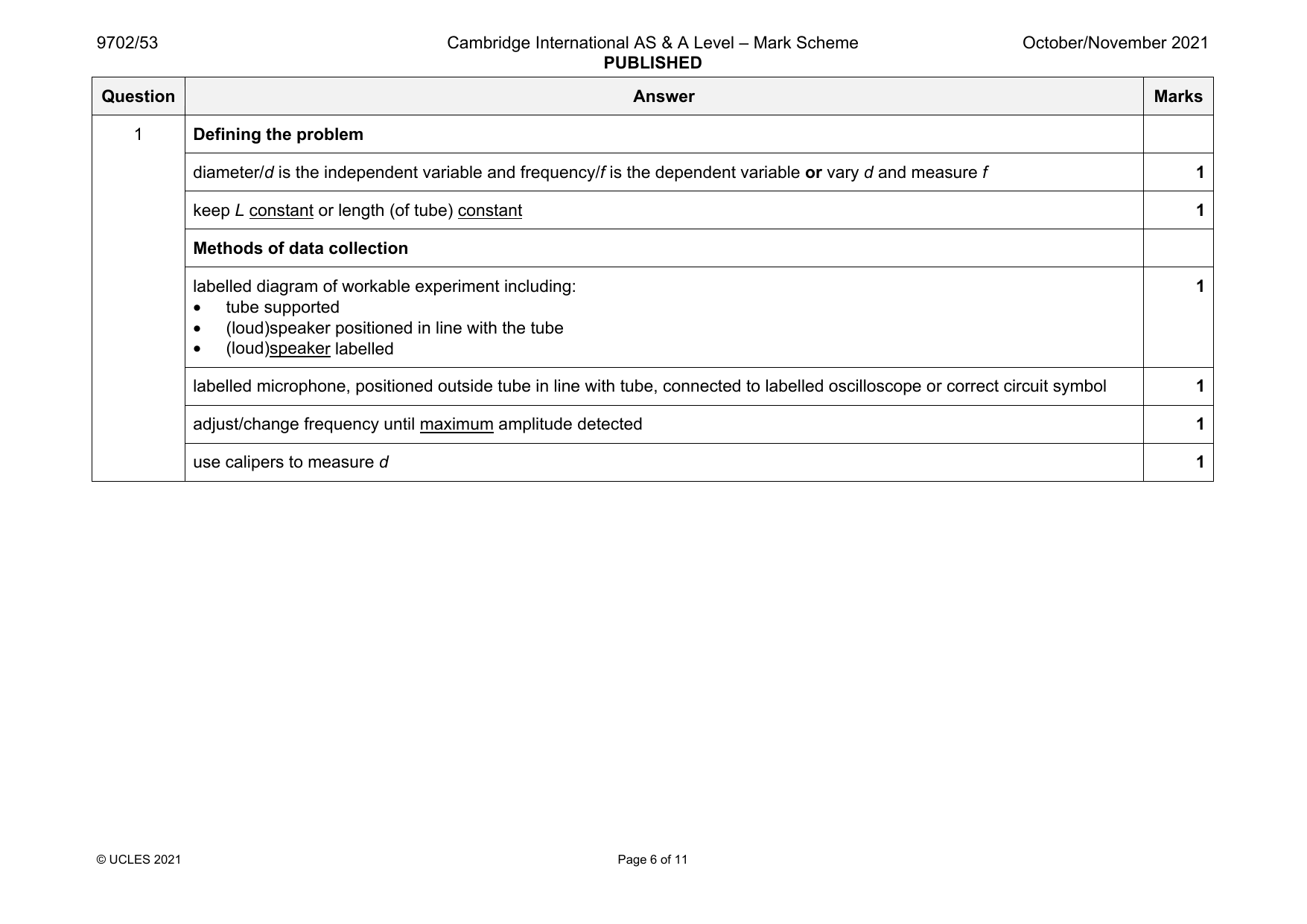
diameter/d is the independent variable and frequency/f is the dependent variable or vary d and measure f 1
keep L constant or length (of tube) constant 1
Methods of data collection
labelled diagram of workable experiment including: 1
• tube supported
• (loud)speaker positioned in line with the tube
• (loud)speaker labelled
labelled microphone, positioned outside tube in line with tube, connected to labelled oscilloscope or correct circuit symbol 1
adjust/change frequency until maximum amplitude detected 1
use calipers to measure d 1
© UCLES 2021 Page 6 of 11
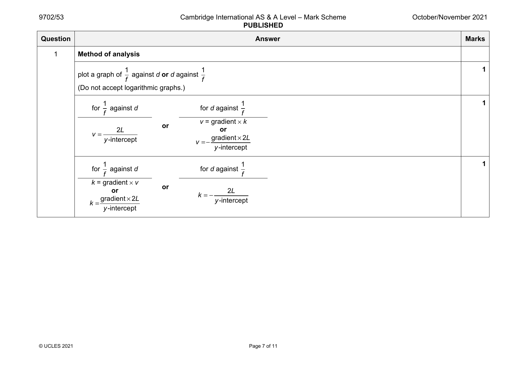
1 Method of analysis
1 1 1
plot a graph of against d or d against
f f
(Do not accept logarithmic graphs.)
1 1 1
for against d for d against
f f
v = gradient × k
or
2L or
v =
y-intercept v = −
gradient×2L
y-intercept
1 1 1
for against d for d against
f f
k = gradient × v
or
or 2L
k =
gradient×2L
k =−
y-intercept
y-intercept
© UCLES 2021 Page 7 of 11
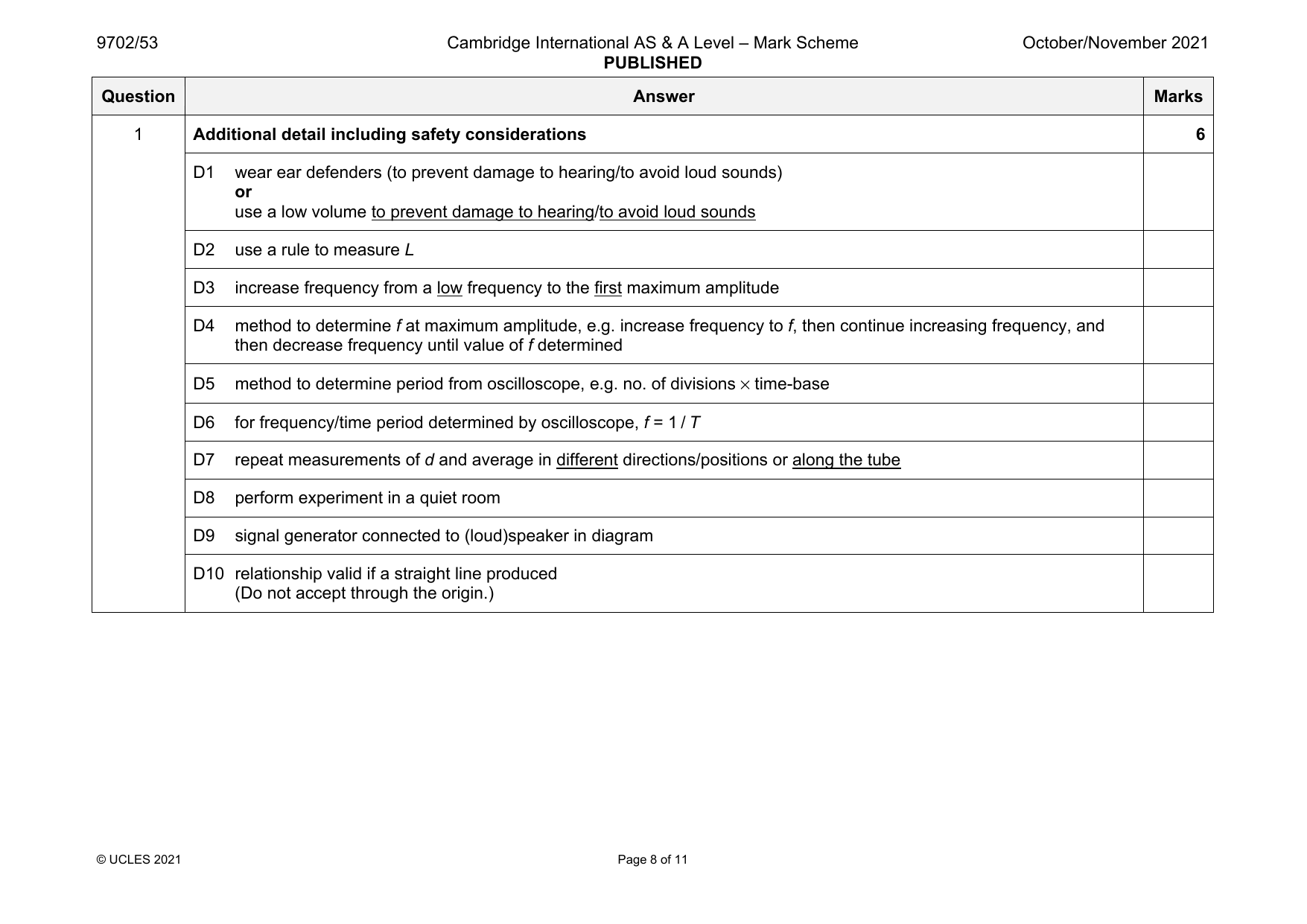
1 Additional detail including safety considerations 6
D1 wear ear defenders (to prevent damage to hearing/to avoid loud sounds)
or
use a low volume to prevent damage to hearing/to avoid loud sounds
D2 use a rule to measure L
D3 increase frequency from a low frequency to the first maximum amplitude
D4 method to determine f at maximum amplitude, e.g. increase frequency to f, then continue increasing frequency, and
then decrease frequency until value of f determined
D5 method to determine period from oscilloscope, e.g. no. of divisions × time-base
D6 for frequency/time period determined by oscilloscope, f = 1 / T
D7 repeat measurements of d and average in different directions/positions or along the tube
D8 perform experiment in a quiet room
D9 signal generator connected to (loud)speaker in diagram
D10 relationship valid if a straight line produced
(Do not accept through the origin.)
© UCLES 2021 Page 8 of 11
Official mark scheme pages: 6, 7, 8 · source PDF URL
9702-2021-on-53-q02
Oct/Nov 2021 · Paper 53 · Question 2 · 15 marks
2(a) t 1
gradient = –
C
y-intercept = ln E
2(b) 1
(R + R ) / kΩ 1
1 2 / 10–6 Ω
R +R
1 2
55 (± 3) 18 or 18.2 ± 0.9
69 (± 3 or 4) 14 or 14.5 ± 0.7
90 (± 4 or 5) 11 or 11.1 ± 0.6
80 (± 4) 13 or 12.5 ± 0.6
101 (± 5) 9.9 or 9.90 or 9.901 ± 0.5
115 (± 6) 8.7 or 8.70 or 8.696 ± 0.4
1
Values of (R + R ) and correct as shown above.
1 2 R +R
1 2
1 1
Absolute uncertainties in from ± 0.9 or ± 1 to ± 0.4 or ± 0.5.
R +R
1 2
2(c)(i) Six points plotted correctly. 1
Must be accurate to half a small square. Diameter of points must be less than half a small square.
1 1
Error bars in plotted correctly.
R +R
1 2
All error bars must be plotted. Total length of bar must be accurate to less than half a small square and symmetrical.
© UCLES 2021 Page 9 of 11
2(c)(ii) Line of best fit drawn. 1
Points must be balanced. Do not accept line from top point to bottom point.
Line must pass between (10.2, 1.10) and (10.8, 1.10) and between (16.7, 0.40) and (17.2, 0.40).
Worst acceptable line drawn (steepest or shallowest possible line that passes through all error bars). 1
All error bars must be plotted.
2(c)(iii) Negative gradient determined with clear substitution of data points into Δy/Δx. 1
Distance between data points must be at least half the length of the drawn line.
Gradient of worst acceptable line determined. 1
uncertainty = (gradient of line of best fit – gradient of worst acceptable line)
or
uncertainty = ½ (steepest worst line gradient – shallowest worst line gradient)
2(c)(iv) y-intercept determined by substitution of point on line into y = mx + c. 1
y-intercept of worst acceptable line determined by substitution of point on line into y = mx + c. 1
uncertainty = y-intercept of line of best fit – y-intercept of worst acceptable line
or
uncertainty = ½ (steepest worst line y-intercept – shallowest worst line y-intercept)
Do not accept ECF from false origin method.
2(d)(i) C determined using gradient and C and E both given to two or three significant figures. 1
t 60
C =− =−
gradient (c)(iii)
E determined using y-intercept and C and E both given with correct SI unit. 1
E =ey-intercept
unit of C: F or C V–1 or s Ω–1
unit of E: V
© UCLES 2021 Page 10 of 11
2(d)(ii) Percentage uncertainty determined with method shown. 1
1 Δgradient
percentage uncertainty = + ×100
60 gradient
Clear substitution must be shown for maximum/minimum methods.
2(e) (R + R ) determined to at least two significant figures from (d)(i) or (c)(iii) and (c)(iv) with correct substitution including 1
1 2
signs and correct power of ten(s).
Do not accept ECF for POT from (c)(iii), (c)(iv) or (d).
( R +R )=− t × 1 = − 60 × 1
1 2 C V C lnV −lnE
ln
E
or
( R +R )= gradient = (c)(iii)
1 2 ln5.0−y-intercept 1.61−(c)(iv)
© UCLES 2021 Page 11 of 11
Official mark scheme pages: 9, 10, 11 · source PDF URL
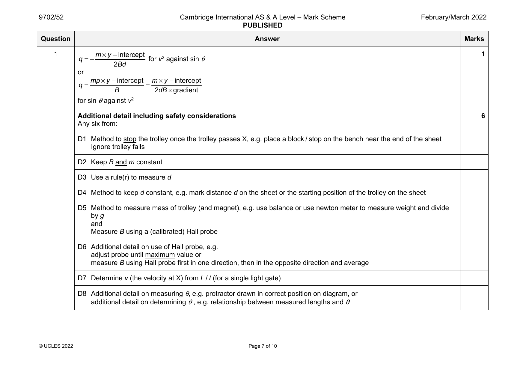
9702-2022-m-52-q01
March 2022 · Paper 52 · Question 1 · 15 marks
1 Defining the problem 1
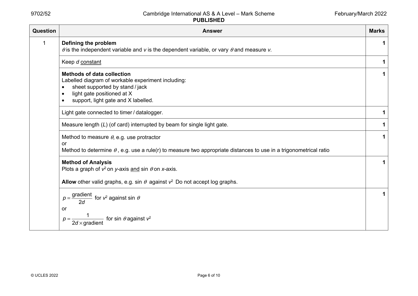
θ is the independent variable and v is the dependent variable, or vary θ and measure v.
Keep d constant 1
Methods of data collection 1
Labelled diagram of workable experiment including:
• sheet supported by stand / jack
• light gate positioned at X
• support, light gate and X labelled.
Light gate connected to timer / datalogger. 1
Measure length (L) (of card) interrupted by beam for single light gate. 1
Method to measure θ, e.g. use protractor 1
or
Method to determine θ , e.g. use a rule(r) to measure two appropriate distances to use in a trigonometrical ratio
Method of Analysis 1
Plots a graph of v2on y-axis and sin θ on x-axis.
Allow other valid graphs, e.g. sin θ against v2 Do not accept log graphs.
gradient 1
p= for v2 against sin θ
2d
or
1
p= for sin θ against v2
2d×gradient
© UCLES 2022 Page 6 of 10
1 m×y −intercept 1
q =− for v2 against sin θ
2Bd
or
mp×y −intercept m×y −intercept
q = =
B 2dB×gradient
for sin θ against v2
Additional detail including safety considerations 6
Any six from:
D1 Method to stop the trolley once the trolley passes X, e.g. place a block / stop on the bench near the end of the sheet
Ignore trolley falls
D2 Keep B and m constant
D3 Use a rule(r) to measure d
D4 Method to keep d constant, e.g. mark distance d on the sheet or the starting position of the trolley on the sheet
D5 Method to measure mass of trolley (and magnet), e.g. use balance or use newton meter to measure weight and divide
by g
and
Measure B using a (calibrated) Hall probe
D6 Additional detail on use of Hall probe, e.g.
adjust probe until maximum value or
measure B using Hall probe first in one direction, then in the opposite direction and average
D7 Determine v (the velocity at X) from L / t (for a single light gate)
D8 Additional detail on measuring θ, e.g. protractor drawn in correct position on diagram, or
additional detail on determining θ , e.g. relationship between measured lengths and θ
© UCLES 2022 Page 7 of 10
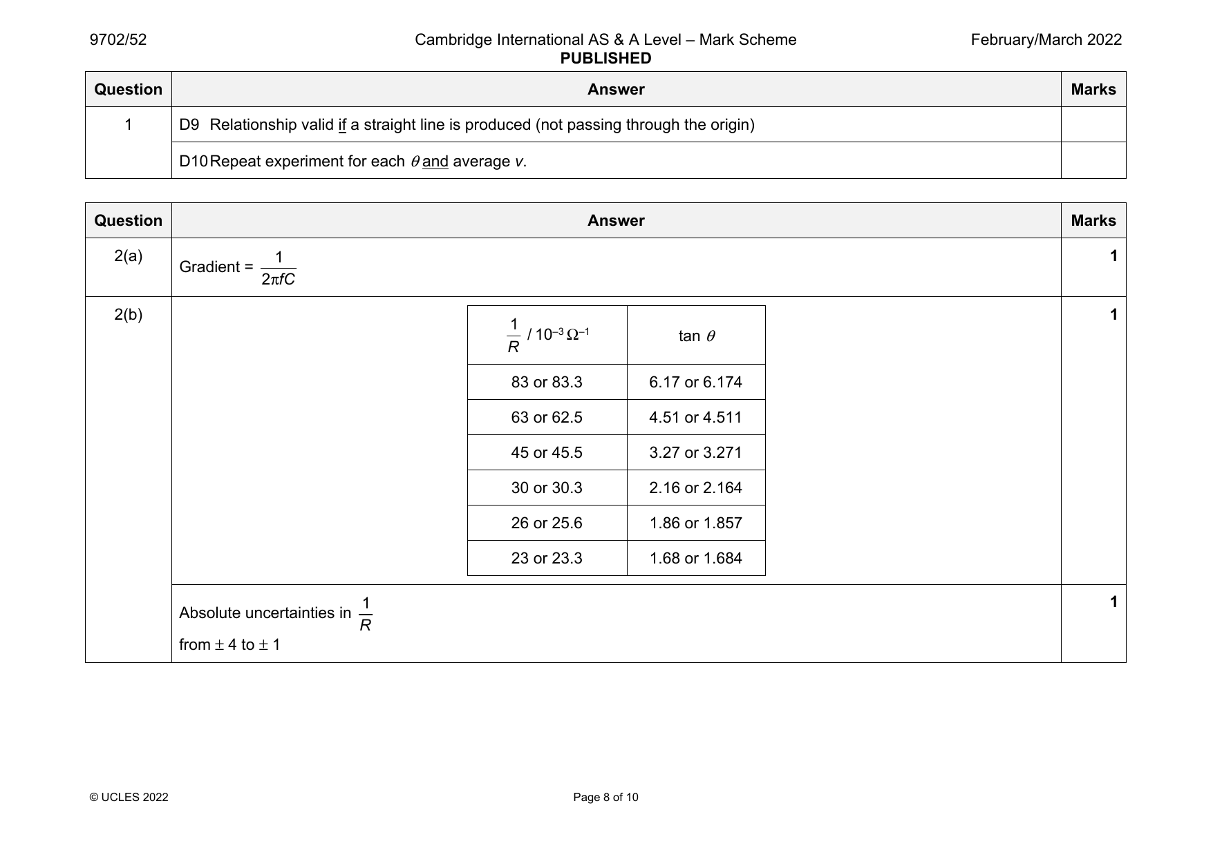
1 D9 Relationship valid if a straight line is produced (not passing through the origin)
D10 Repeat experiment for each θ and average v.
Question Answer Marks
Official mark scheme pages: 6, 7, 8 · source PDF URL
9702-2022-m-52-q02
March 2022 · Paper 52 · Question 2 · 15 marks
2(a) 1 1
Gradient =
2πfC
2(b) 1
1
/ 10–3 Ω–1 tan θ
R
83 or 83.3 6.17 or 6.174
63 or 62.5 4.51 or 4.511
45 or 45.5 3.27 or 3.271
30 or 30.3 2.16 or 2.164
26 or 25.6 1.86 or 1.857
23 or 23.3 1.68 or 1.684
1 1
Absolute uncertainties in
R
from ± 4 to ± 1
© UCLES 2022 Page 8 of 10
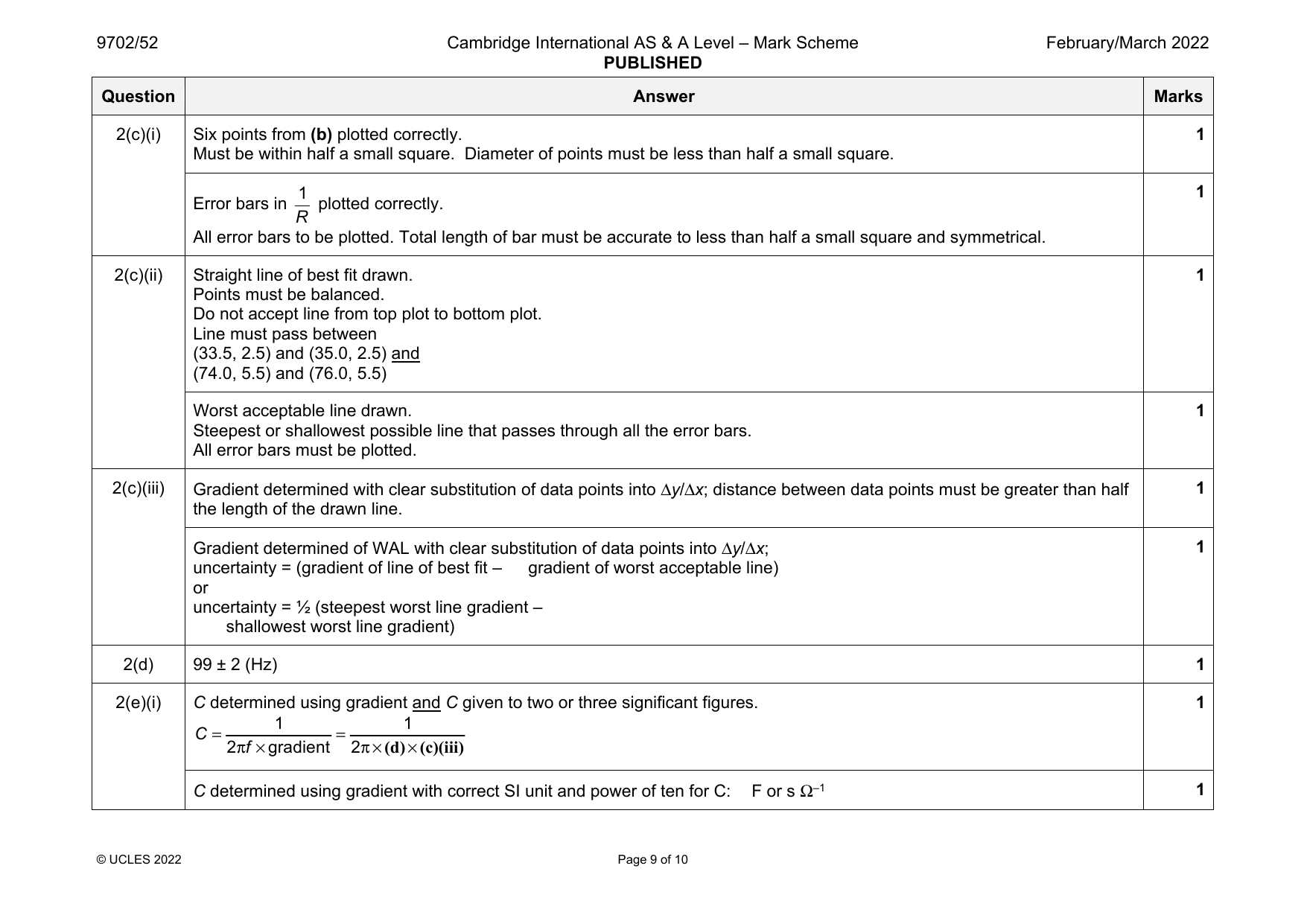
2(c)(i) Six points from (b) plotted correctly. 1
Must be within half a small square. Diameter of points must be less than half a small square.
1 1
Error bars in plotted correctly.
R
All error bars to be plotted. Total length of bar must be accurate to less than half a small square and symmetrical.
2(c)(ii) Straight line of best fit drawn. 1
Points must be balanced.
Do not accept line from top plot to bottom plot.
Line must pass between
(33.5, 2.5) and (35.0, 2.5) and
(74.0, 5.5) and (76.0, 5.5)
Worst acceptable line drawn. 1
Steepest or shallowest possible line that passes through all the error bars.
All error bars must be plotted.
2(c)(iii) Gradient determined with clear substitution of data points into Δy/Δx; distance between data points must be greater than half 1
the length of the drawn line.
Gradient determined of WAL with clear substitution of data points into Δy/Δx; 1
uncertainty = (gradient of line of best fit – gradient of worst acceptable line)
or
uncertainty = ½ (steepest worst line gradient –
shallowest worst line gradient)
2(d) 99 ± 2 (Hz) 1
2(e)(i) C determined using gradient and C given to two or three significant figures. 1
1 1
C = =
2πf ×gradient 2π×(d)×(c)(iii)
C determined using gradient with correct SI unit and power of ten for C: F or s Ω–1 1
© UCLES 2022 Page 9 of 10
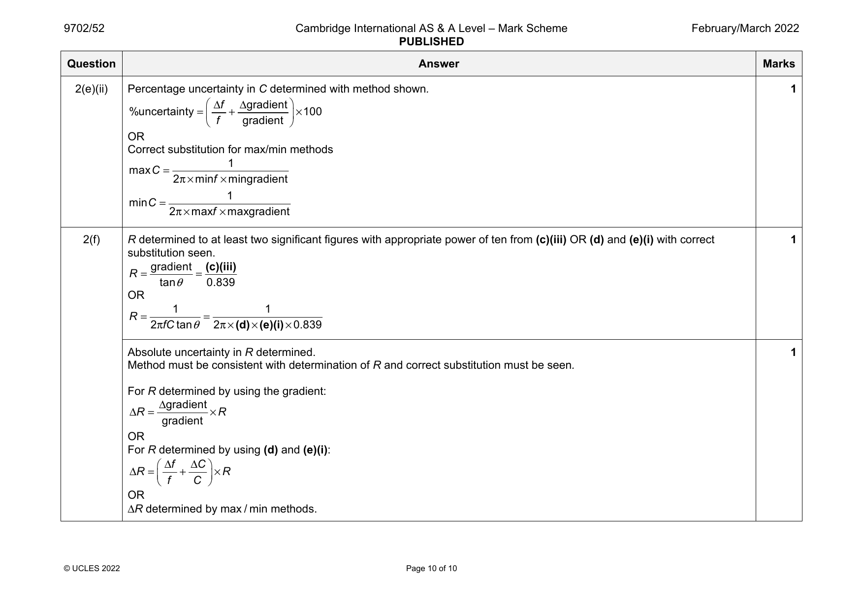
2(e)(ii) Percentage uncertainty in C determined with method shown. 1
Δf Δgradient
%uncertainty = + ×100
f gradient
OR
Correct substitution for max/min methods
1
maxC =
2π×minf ×mingradient
1
minC =
2π×maxf ×maxgradient
2(f) R determined to at least two significant figures with appropriate power of ten from (c)(iii) OR (d) and (e)(i) with correct 1
substitution seen.
gradient (c)(iii)
R = =
tanθ 0.839
OR
1 1
R = =
2πfCtanθ 2π×(d)×(e)(i)×0.839
Absolute uncertainty in R determined. 1
Method must be consistent with determination of R and correct substitution must be seen.
For R determined by using the gradient:
Δgradient
ΔR = ×R
gradient
OR
For R determined by using (d) and (e)(i):
Δf ΔC
ΔR = + ×R
f C
OR
ΔR determined by max / min methods.
© UCLES 2022 Page 10 of 10
Official mark scheme pages: 8, 9, 10 · source PDF URL
9702-2022-mj-51-q01
May/June 2022 · Paper 51 · Question 1 · 15 marks
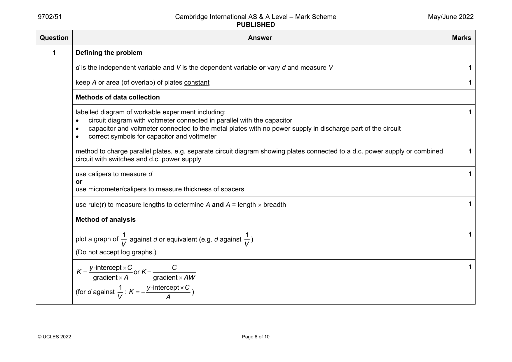
1 Defining the problem
d is the independent variable and V is the dependent variable or vary d and measure V 1
keep A or area (of overlap) of plates constant 1
Methods of data collection
labelled diagram of workable experiment including: 1
circuit diagram with voltmeter connected in parallel with the capacitor
capacitor and voltmeter connected to the metal plates with no power supply in discharge part of the circuit
correct symbols for capacitor and voltmeter
method to charge parallel plates, e.g. separate circuit diagram showing plates connected to a d.c. power supply or combined 1
circuit with switches and d.c. power supply
use calipers to measure d 1
or
use micrometer/calipers to measure thickness of spacers
use rule(r) to measure lengths to determine A and A = length breadth 1
Method of analysis
1 1 1
plot a graph of against d or equivalent (e.g. d against )
V V
(Do not accept log graphs.)
y-interceptC C 1
K or K
gradientA gradientAW
1 y-interceptC
(for d against : K )
V A
© UCLES 2022 Page 6 of 10
1 1 1
W
y-intercept
1 gradient gradientC
(for d against : W or W )
V y-intercept AK
Additional detail including safety considerations 6
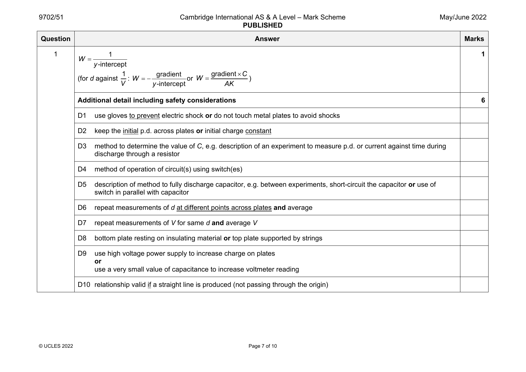
D1 use gloves to prevent electric shock or do not touch metal plates to avoid shocks
D2 keep the initial p.d. across plates or initial charge constant
D3 method to determine the value of C, e.g. description of an experiment to measure p.d. or current against time during
discharge through a resistor
D4 method of operation of circuit(s) using switch(es)
D5 description of method to fully discharge capacitor, e.g. between experiments, short-circuit the capacitor or use of
switch in parallel with capacitor
D6 repeat measurements of d at different points across plates and average
D7 repeat measurements of V for same d and average V
D8 bottom plate resting on insulating material or top plate supported by strings
D9 use high voltage power supply to increase charge on plates
or
use a very small value of capacitance to increase voltmeter reading
D10 relationship valid if a straight line is produced (not passing through the origin)
© UCLES 2022 Page 7 of 10
Official mark scheme pages: 6, 7 · source PDF URL
9702-2022-mj-51-q02
May/June 2022 · Paper 51 · Question 2 · 15 marks
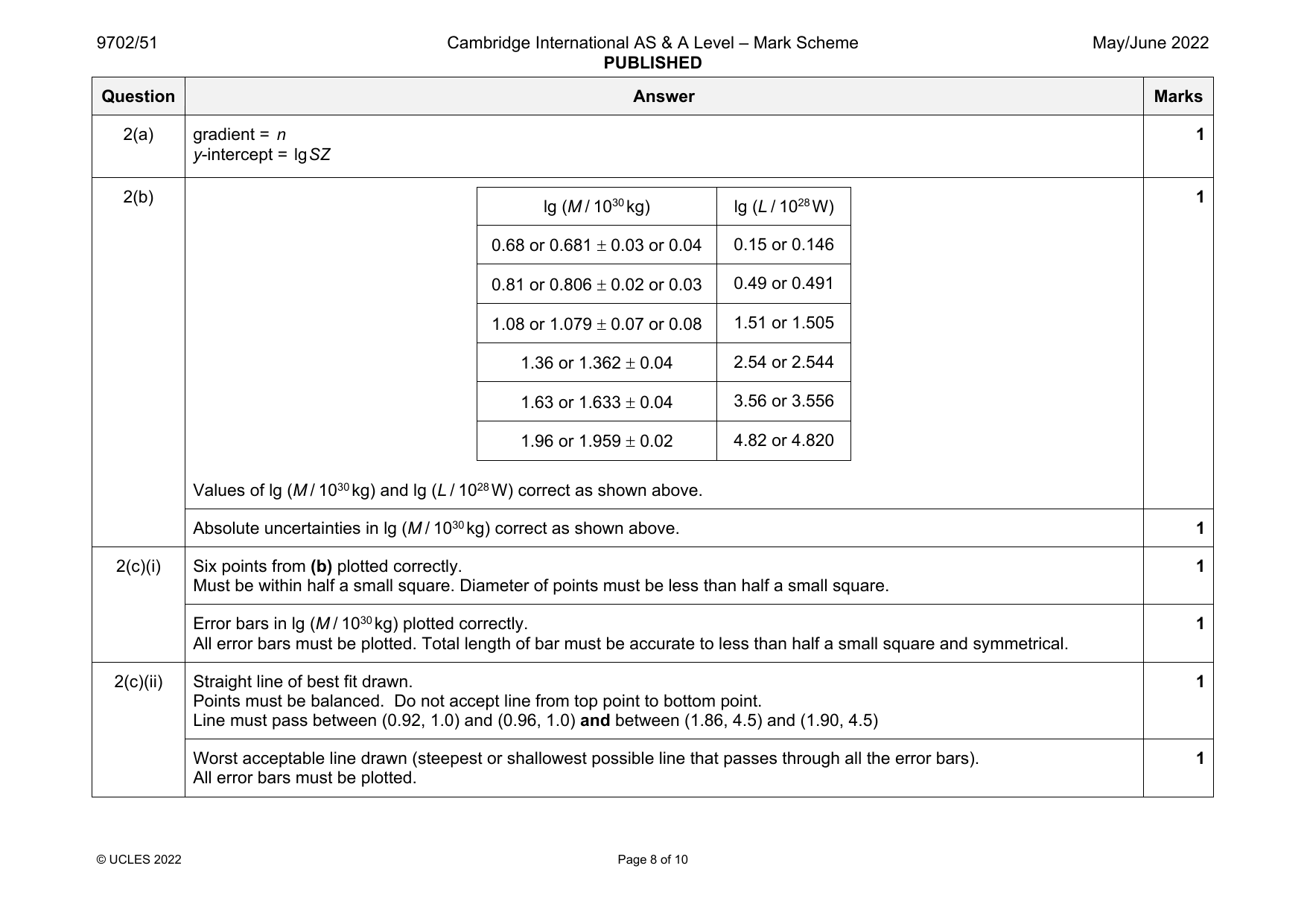
2(a) gradient = n 1
y-intercept = lgSZ
2(b) 1
lg (M / 1030kg) lg (L / 1028W)
0.68 or 0.681 0.03 or 0.04 0.15 or 0.146
0.81 or 0.806 0.02 or 0.03 0.49 or 0.491
1.08 or 1.079 0.07 or 0.08 1.51 or 1.505
1.36 or 1.362 0.04 2.54 or 2.544
1.63 or 1.633 0.04 3.56 or 3.556
1.96 or 1.959 0.02 4.82 or 4.820
Values of lg (M / 1030kg) and lg (L / 1028W) correct as shown above.
Absolute uncertainties in lg (M / 1030kg) correct as shown above. 1
2(c)(i) Six points from (b) plotted correctly. 1
Must be within half a small square. Diameter of points must be less than half a small square.
Error bars in lg (M / 1030kg) plotted correctly. 1
All error bars must be plotted. Total length of bar must be accurate to less than half a small square and symmetrical.
2(c)(ii) Straight line of best fit drawn. 1
Points must be balanced. Do not accept line from top point to bottom point.
Line must pass between (0.92, 1.0) and (0.96, 1.0) and between (1.86, 4.5) and (1.90, 4.5)
Worst acceptable line drawn (steepest or shallowest possible line that passes through all the error bars). 1
All error bars must be plotted.
© UCLES 2022 Page 8 of 10
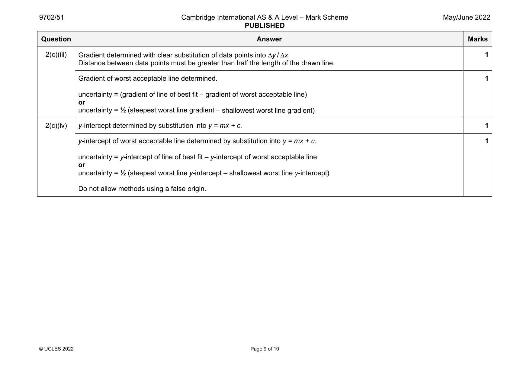
2(c)(iii) Gradient determined with clear substitution of data points into y / x. 1
Distance between data points must be greater than half the length of the drawn line.
Gradient of worst acceptable line determined. 1
uncertainty = (gradient of line of best fit – gradient of worst acceptable line)
or
uncertainty = ½ (steepest worst line gradient – shallowest worst line gradient)
2(c)(iv) y-intercept determined by substitution into y = mx + c. 1
y-intercept of worst acceptable line determined by substitution into y = mx + c. 1
uncertainty = y-intercept of line of best fit – y-intercept of worst acceptable line
or
uncertainty = ½ (steepest worst line y-intercept – shallowest worst line y-intercept)
Do not allow methods using a false origin.
© UCLES 2022 Page 9 of 10
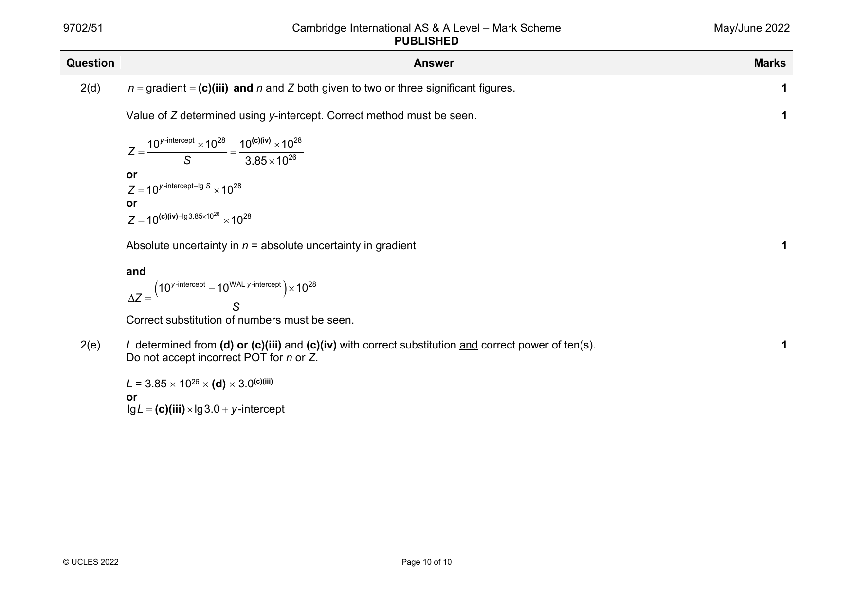
2(d) n gradient (c)(iii) and n and Z both given to two or three significant figures. 1
Value of Z determined using y-intercept. Correct method must be seen. 1
10y-intercept 1028 10(c)(iv)1028
Z
S 3.851026
or
Z 10y-interceptlg S 1028
or
Z 10(c)(iv)lg 3.851026 1028
Absolute uncertainty in n = absolute uncertainty in gradient 1
and
10y-intercept 10WAL y-intercept 1028
Z
S
Correct substitution of numbers must be seen.
2(e) L determined from (d) or (c)(iii) and (c)(iv) with correct substitution and correct power of ten(s). 1
Do not accept incorrect POT for n or Z.
L = 3.85 1026 (d) 3.0(c)(iii)
or
lgL(c)(iii)lg3.0y-intercept
© UCLES 2022 Page 10 of 10
Official mark scheme pages: 8, 9, 10 · source PDF URL
9702-2022-mj-52-q01
May/June 2022 · Paper 52 · Question 1 · 15 marks
1 Defining the problem
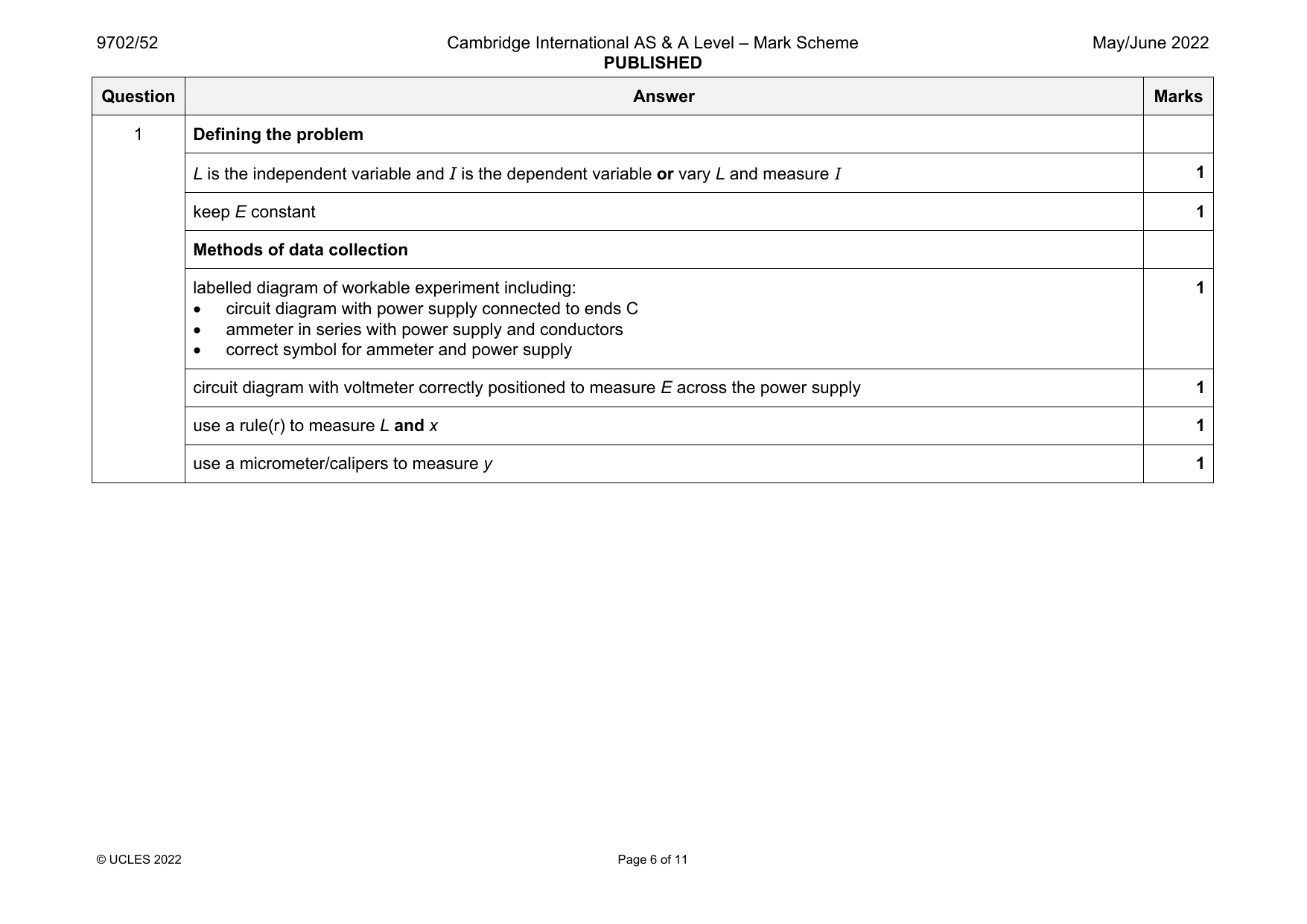
L is the independent variable and I is the dependent variable or vary L and measure I 1
keep E constant 1
Methods of data collection
labelled diagram of workable experiment including: 1
circuit diagram with power supply connected to ends C
ammeter in series with power supply and conductors
correct symbol for ammeter and power supply
circuit diagram with voltmeter correctly positioned to measure E across the power supply 1
use a rule(r) to measure L and x 1
use a micrometer/calipers to measure y 1
© UCLES 2022 Page 6 of 11
1 Method of analysis
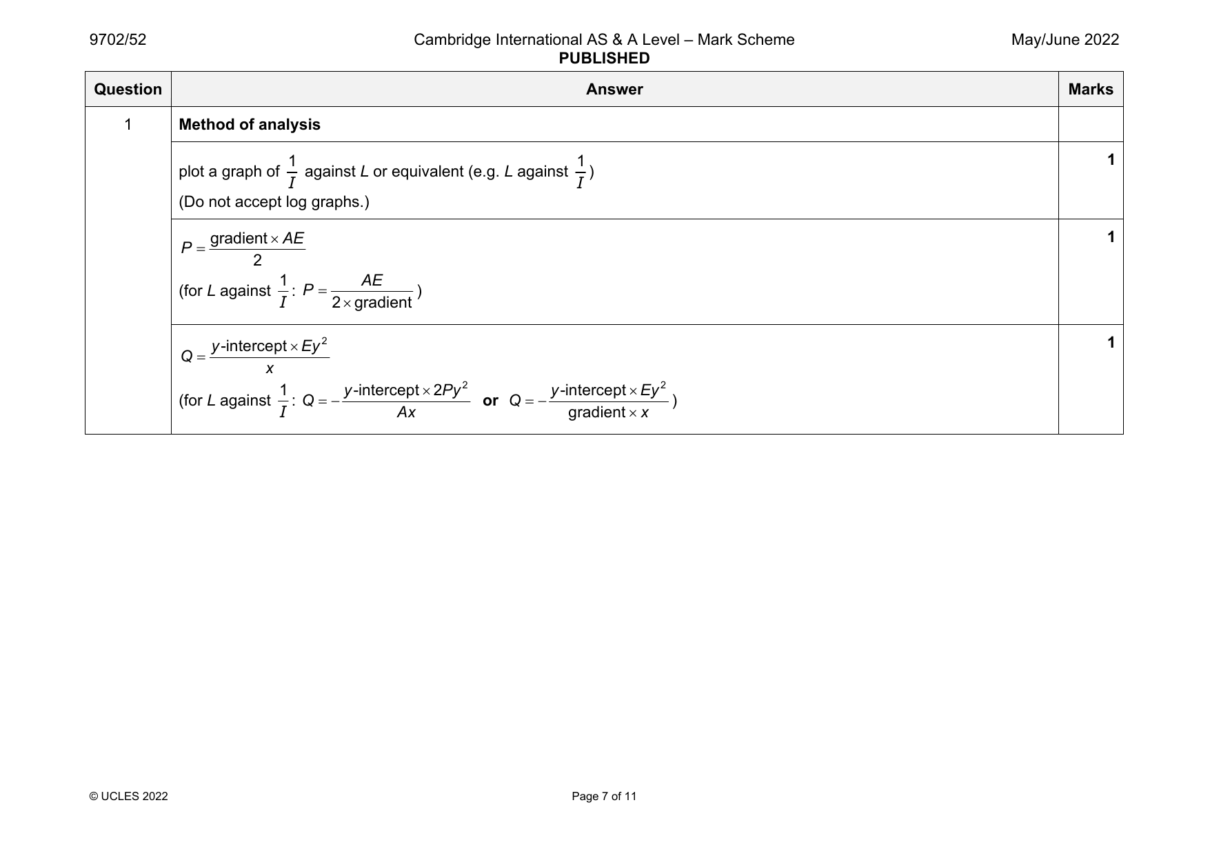
1 1 1
plot a graph of against L or equivalent (e.g. L against )
I I
(Do not accept log graphs.)
gradientAE 1
P
Official mark scheme pages: 6, 7 · source PDF URL
9702-2022-mj-52-q02
May/June 2022 · Paper 52 · Question 2 · 15 marks
2
1 AE
(for L against : P )
I 2gradient
y-interceptEy2 1
Q
x
1 y-intercept2Py2 y-interceptEy2
(for L against : Q or Q )
I Ax gradientx
© UCLES 2022 Page 7 of 11
9702/52 Cambridge International AS & A Level – Mark Scheme May/June 2022
PUBLISHED
Question Answer Marks
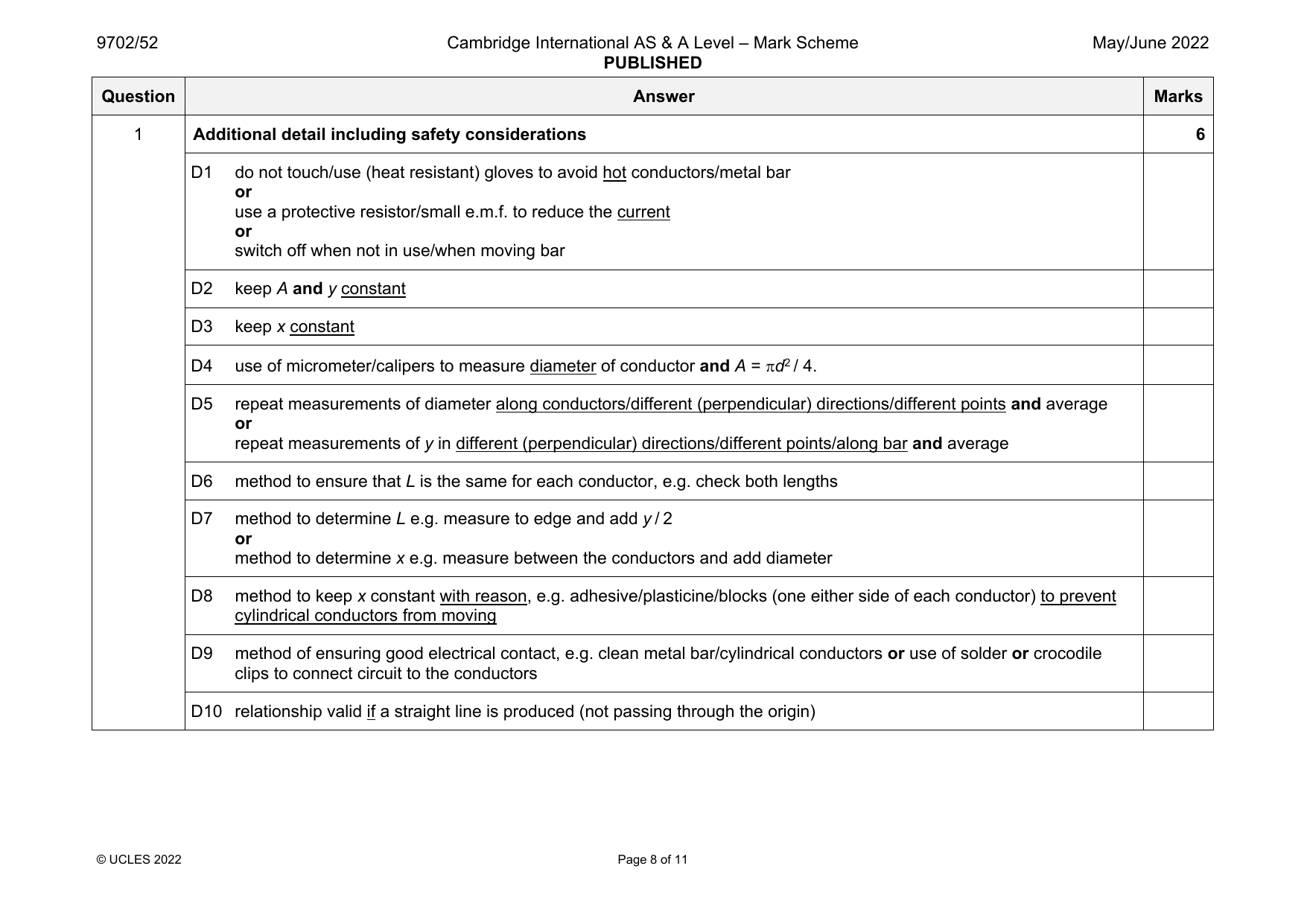
1 Additional detail including safety considerations 6
D1 do not touch/use (heat resistant) gloves to avoid hot conductors/metal bar
or
use a protective resistor/small e.m.f. to reduce the current
or
switch off when not in use/when moving bar
D2 keep A and y constant
D3 keep x constant
D4 use of micrometer/calipers to measure diameter of conductor and A = d2 / 4.
D5 repeat measurements of diameter along conductors/different (perpendicular) directions/different points and average
or
repeat measurements of y in different (perpendicular) directions/different points/along bar and average
D6 method to ensure that L is the same for each conductor, e.g. check both lengths
D7 method to determine L e.g. measure to edge and add y / 2
or
method to determine x e.g. measure between the conductors and add diameter
D8 method to keep x constant with reason, e.g. adhesive/plasticine/blocks (one either side of each conductor) to prevent
cylindrical conductors from moving
D9 method of ensuring good electrical contact, e.g. clean metal bar/cylindrical conductors or use of solder or crocodile
clips to connect circuit to the conductors
D10 relationship valid if a straight line is produced (not passing through the origin)
© UCLES 2022 Page 8 of 11
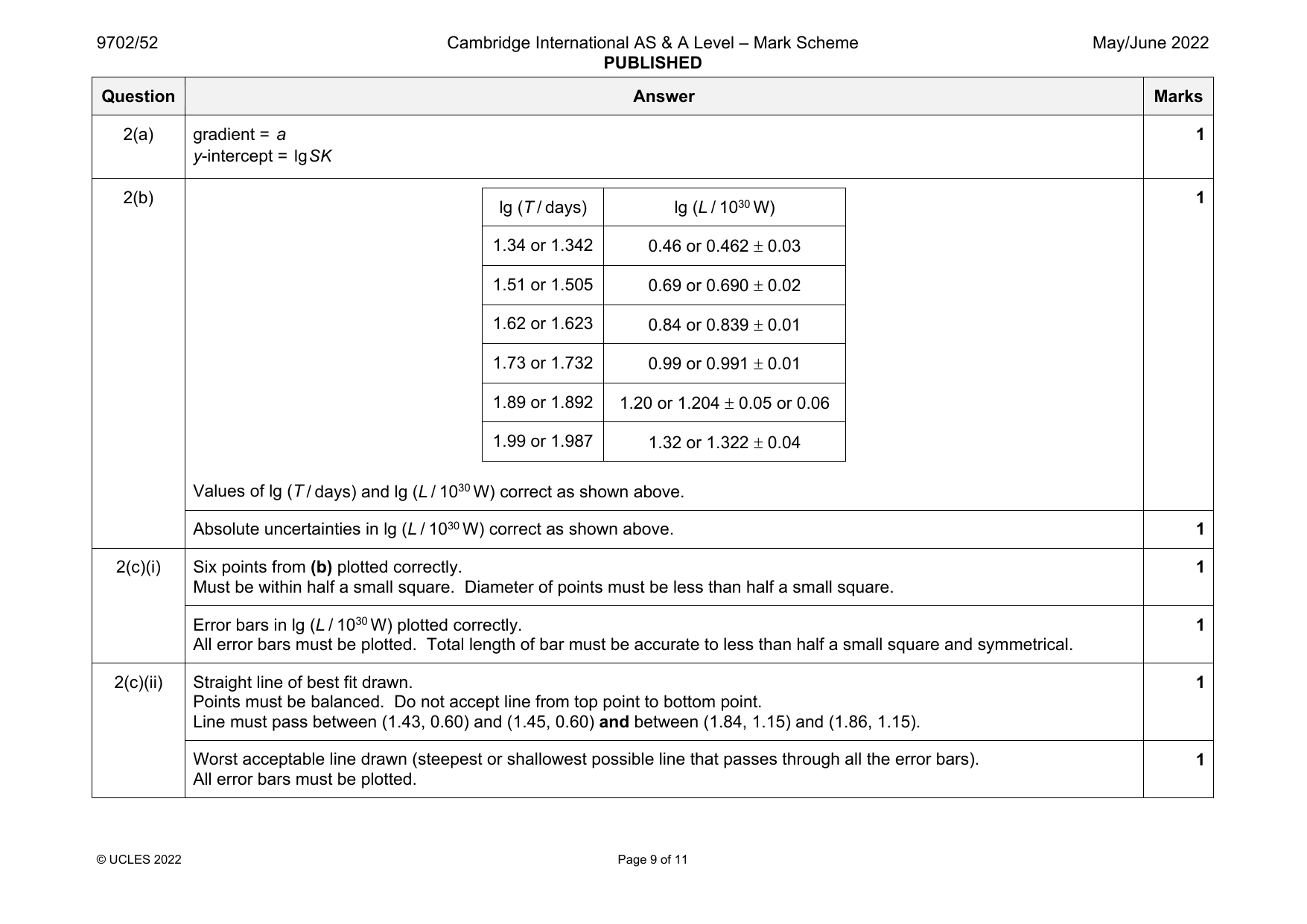
2(a) gradient = a 1
y-intercept = lgSK
2(b) 1
lg (T / days) lg (L / 1030W)
1.34 or 1.342 0.46 or 0.462 0.03
1.51 or 1.505 0.69 or 0.690 0.02
1.62 or 1.623 0.84 or 0.839 0.01
1.73 or 1.732 0.99 or 0.991 0.01
1.89 or 1.892 1.20 or 1.204 0.05 or 0.06
1.99 or 1.987 1.32 or 1.322 0.04
Values of lg (T / days) and lg (L / 1030W) correct as shown above.
Absolute uncertainties in lg (L / 1030W) correct as shown above. 1
2(c)(i) Six points from (b) plotted correctly. 1
Must be within half a small square. Diameter of points must be less than half a small square.
Error bars in lg (L / 1030W) plotted correctly. 1
All error bars must be plotted. Total length of bar must be accurate to less than half a small square and symmetrical.
2(c)(ii) Straight line of best fit drawn. 1
Points must be balanced. Do not accept line from top point to bottom point.
Line must pass between (1.43, 0.60) and (1.45, 0.60) and between (1.84, 1.15) and (1.86, 1.15).
Worst acceptable line drawn (steepest or shallowest possible line that passes through all the error bars). 1
All error bars must be plotted.
© UCLES 2022 Page 9 of 11
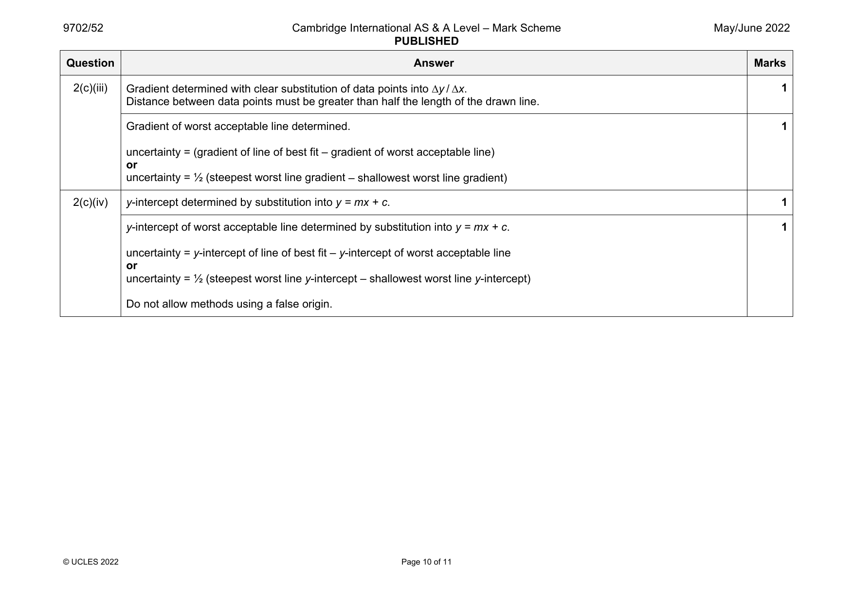
2(c)(iii) Gradient determined with clear substitution of data points into y / x. 1
Distance between data points must be greater than half the length of the drawn line.
Gradient of worst acceptable line determined. 1
uncertainty = (gradient of line of best fit – gradient of worst acceptable line)
or
uncertainty = ½ (steepest worst line gradient – shallowest worst line gradient)
2(c)(iv) y-intercept determined by substitution into y = mx + c. 1
y-intercept of worst acceptable line determined by substitution into y = mx + c. 1
uncertainty = y-intercept of line of best fit – y-intercept of worst acceptable line
or
uncertainty = ½ (steepest worst line y-intercept – shallowest worst line y-intercept)
Do not allow methods using a false origin.
© UCLES 2022 Page 10 of 11
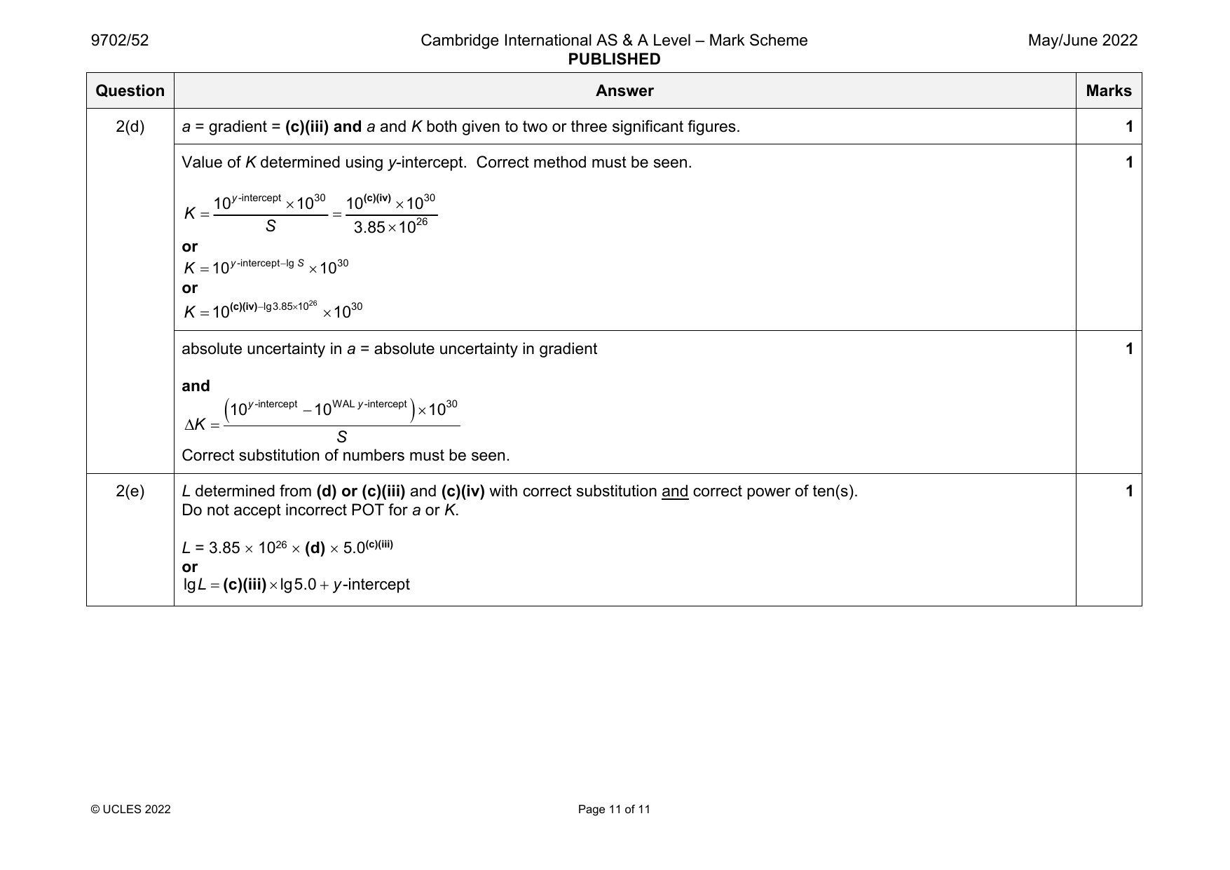
2(d) a = gradient = (c)(iii) and a and K both given to two or three significant figures. 1
Value of K determined using y-intercept. Correct method must be seen. 1
10y-intercept 1030 10(c)(iv)1030
K
S 3.851026
or
K 10y-interceptlg S 1030
or
K 10(c)(iv)lg 3.851026 1030
absolute uncertainty in a = absolute uncertainty in gradient 1
and
10y-intercept 10WAL y-intercept 1030
K
S
Correct substitution of numbers must be seen.
2(e) L determined from (d) or (c)(iii) and (c)(iv) with correct substitution and correct power of ten(s). 1
Do not accept incorrect POT for a or K.
L = 3.85 1026 (d) 5.0(c)(iii)
or
lgL(c)(iii)lg5.0y-intercept
© UCLES 2022 Page 11 of 11
Official mark scheme pages: 7, 8, 9, 10, 11 · source PDF URL
9702-2022-mj-53-q01
May/June 2022 · Paper 53 · Question 1 · 15 marks
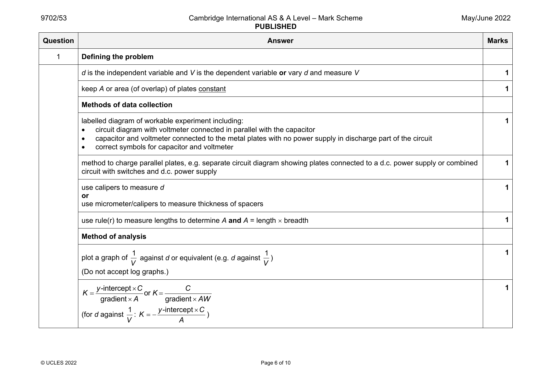
1 Defining the problem
d is the independent variable and V is the dependent variable or vary d and measure V 1
keep A or area (of overlap) of plates constant 1
Methods of data collection
labelled diagram of workable experiment including: 1
circuit diagram with voltmeter connected in parallel with the capacitor
capacitor and voltmeter connected to the metal plates with no power supply in discharge part of the circuit
correct symbols for capacitor and voltmeter
method to charge parallel plates, e.g. separate circuit diagram showing plates connected to a d.c. power supply or combined 1
circuit with switches and d.c. power supply
use calipers to measure d 1
or
use micrometer/calipers to measure thickness of spacers
use rule(r) to measure lengths to determine A and A = length breadth 1
Method of analysis
1 1 1
plot a graph of against d or equivalent (e.g. d against )
V V
(Do not accept log graphs.)
y-interceptC C 1
K or K
gradientA gradientAW
1 y-interceptC
(for d against : K )
V A
© UCLES 2022 Page 6 of 10
1 1 1
W
y-intercept
1 gradient gradientC
(for d against : W or W )
V y-intercept AK
Additional detail including safety considerations 6
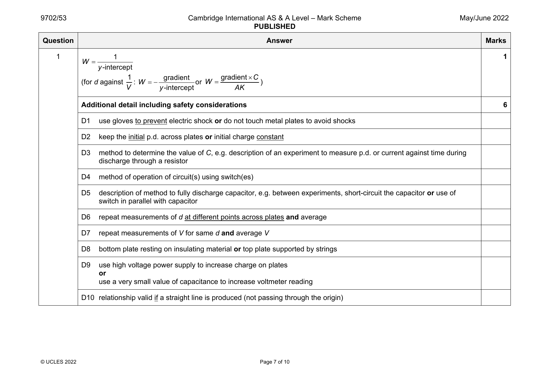
D1 use gloves to prevent electric shock or do not touch metal plates to avoid shocks
D2 keep the initial p.d. across plates or initial charge constant
D3 method to determine the value of C, e.g. description of an experiment to measure p.d. or current against time during
discharge through a resistor
D4 method of operation of circuit(s) using switch(es)
D5 description of method to fully discharge capacitor, e.g. between experiments, short-circuit the capacitor or use of
switch in parallel with capacitor
D6 repeat measurements of d at different points across plates and average
D7 repeat measurements of V for same d and average V
D8 bottom plate resting on insulating material or top plate supported by strings
D9 use high voltage power supply to increase charge on plates
or
use a very small value of capacitance to increase voltmeter reading
D10 relationship valid if a straight line is produced (not passing through the origin)
© UCLES 2022 Page 7 of 10
Official mark scheme pages: 6, 7 · source PDF URL
9702-2022-mj-53-q02
May/June 2022 · Paper 53 · Question 2 · 15 marks
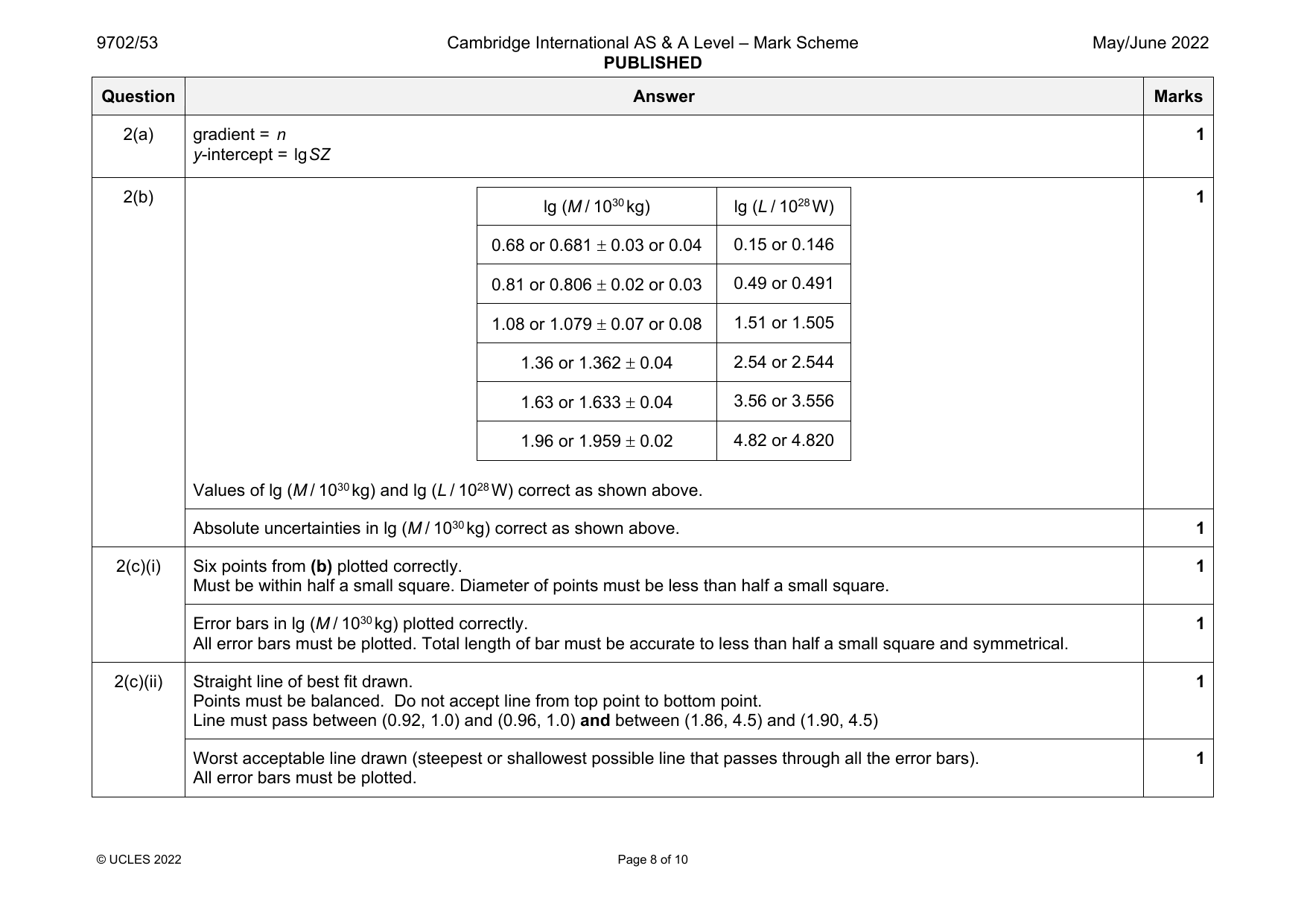
2(a) gradient = n 1
y-intercept = lgSZ
2(b) 1
lg (M / 1030kg) lg (L / 1028W)
0.68 or 0.681 0.03 or 0.04 0.15 or 0.146
0.81 or 0.806 0.02 or 0.03 0.49 or 0.491
1.08 or 1.079 0.07 or 0.08 1.51 or 1.505
1.36 or 1.362 0.04 2.54 or 2.544
1.63 or 1.633 0.04 3.56 or 3.556
1.96 or 1.959 0.02 4.82 or 4.820
Values of lg (M / 1030kg) and lg (L / 1028W) correct as shown above.
Absolute uncertainties in lg (M / 1030kg) correct as shown above. 1
2(c)(i) Six points from (b) plotted correctly. 1
Must be within half a small square. Diameter of points must be less than half a small square.
Error bars in lg (M / 1030kg) plotted correctly. 1
All error bars must be plotted. Total length of bar must be accurate to less than half a small square and symmetrical.
2(c)(ii) Straight line of best fit drawn. 1
Points must be balanced. Do not accept line from top point to bottom point.
Line must pass between (0.92, 1.0) and (0.96, 1.0) and between (1.86, 4.5) and (1.90, 4.5)
Worst acceptable line drawn (steepest or shallowest possible line that passes through all the error bars). 1
All error bars must be plotted.
© UCLES 2022 Page 8 of 10
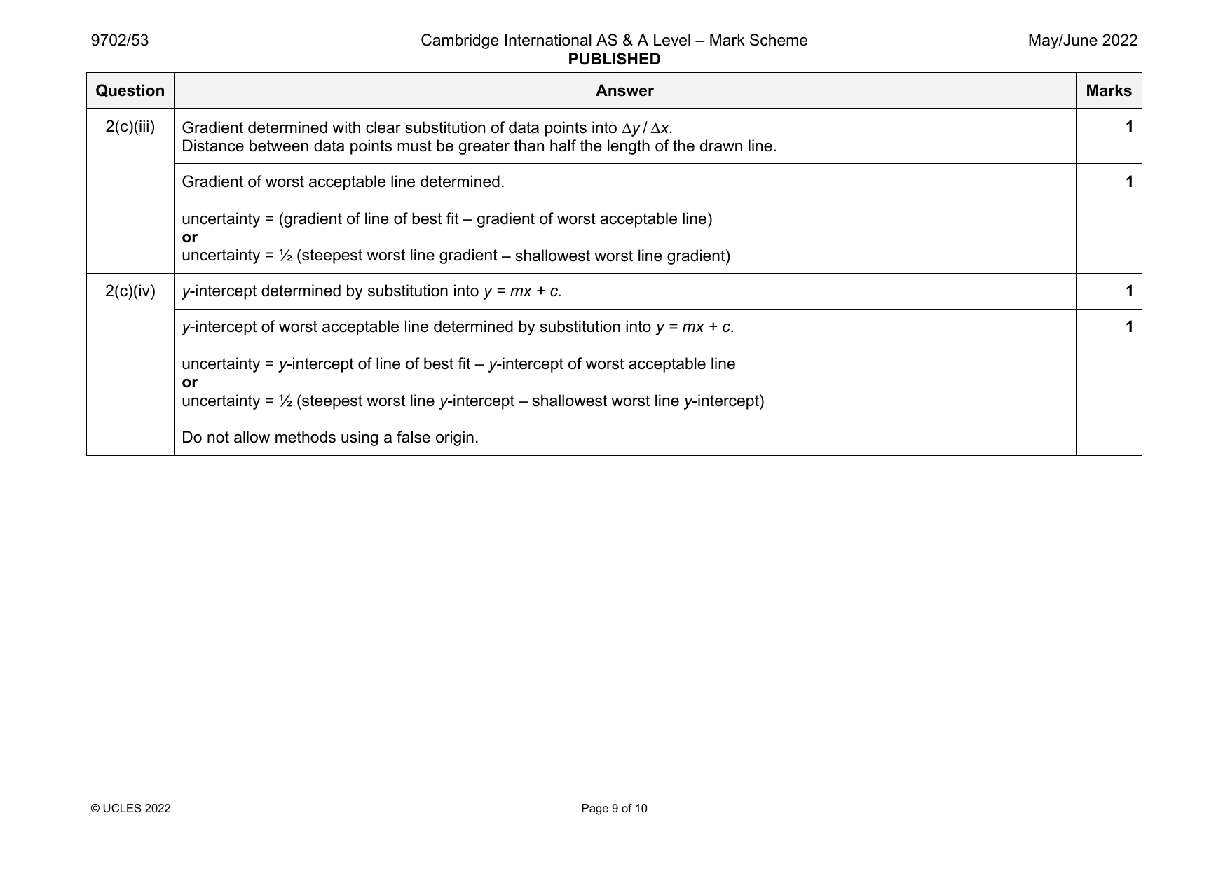
2(c)(iii) Gradient determined with clear substitution of data points into y / x. 1
Distance between data points must be greater than half the length of the drawn line.
Gradient of worst acceptable line determined. 1
uncertainty = (gradient of line of best fit – gradient of worst acceptable line)
or
uncertainty = ½ (steepest worst line gradient – shallowest worst line gradient)
2(c)(iv) y-intercept determined by substitution into y = mx + c. 1
y-intercept of worst acceptable line determined by substitution into y = mx + c. 1
uncertainty = y-intercept of line of best fit – y-intercept of worst acceptable line
or
uncertainty = ½ (steepest worst line y-intercept – shallowest worst line y-intercept)
Do not allow methods using a false origin.
© UCLES 2022 Page 9 of 10
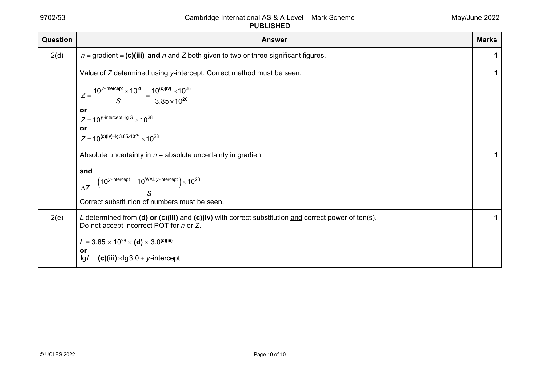
2(d) n gradient (c)(iii) and n and Z both given to two or three significant figures. 1
Value of Z determined using y-intercept. Correct method must be seen. 1
10y-intercept 1028 10(c)(iv)1028
Z
S 3.851026
or
Z 10y-interceptlg S 1028
or
Z 10(c)(iv)lg 3.851026 1028
Absolute uncertainty in n = absolute uncertainty in gradient 1
and
10y-intercept 10WAL y-intercept 1028
Z
S
Correct substitution of numbers must be seen.
2(e) L determined from (d) or (c)(iii) and (c)(iv) with correct substitution and correct power of ten(s). 1
Do not accept incorrect POT for n or Z.
L = 3.85 1026 (d) 3.0(c)(iii)
or
lgL(c)(iii)lg3.0y-intercept
© UCLES 2022 Page 10 of 10
Official mark scheme pages: 8, 9, 10 · source PDF URL
9702-2022-on-51-q01
Oct/Nov 2022 · Paper 51 · Question 1 · 15 marks
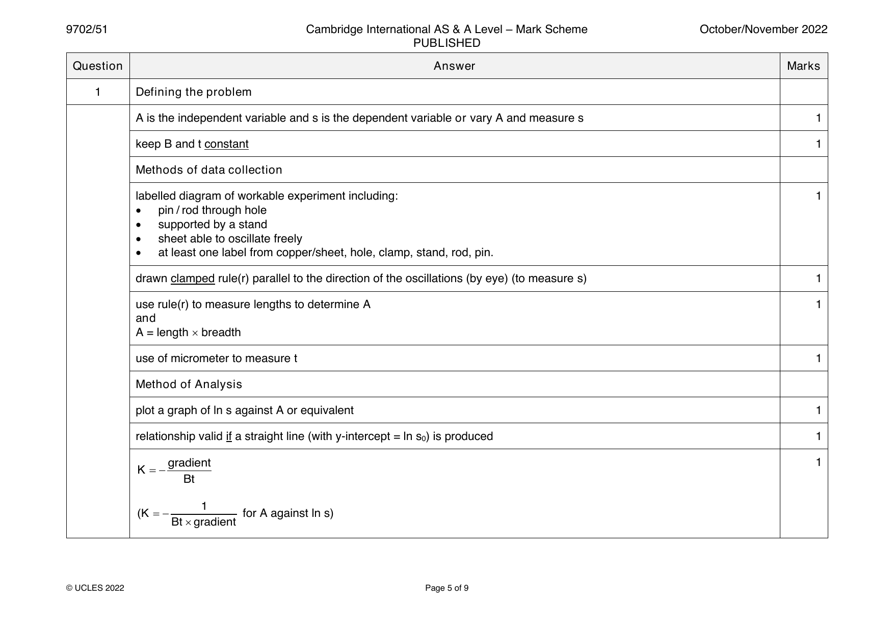
1 Defining the problem
A is the independent variable and s is the dependent variable or vary A and measure s 1
keep B and t constant 1
Methods of data collection
labelled diagram of workable experiment including: 1
• pin / rod through hole
• supported by a stand
• sheet able to oscillate freely
• at least one label from copper/sheet, hole, clamp, stand, rod, pin.
drawn clamped rule(r) parallel to the direction of the oscillations (by eye) (to measure s) 1
use rule(r) to measure lengths to determine A 1
and
A = length breadth
use of micrometer to measure t 1
Method of Analysis
plot a graph of ln s against A or equivalent 1
relationship valid if a straight line (with y-intercept = ln s ) is produced 1
0
gradient 1
K =−
Bt
1
(K =− for A against ln s)
Btgradient
© UCLES 2022 Page 5 of 9
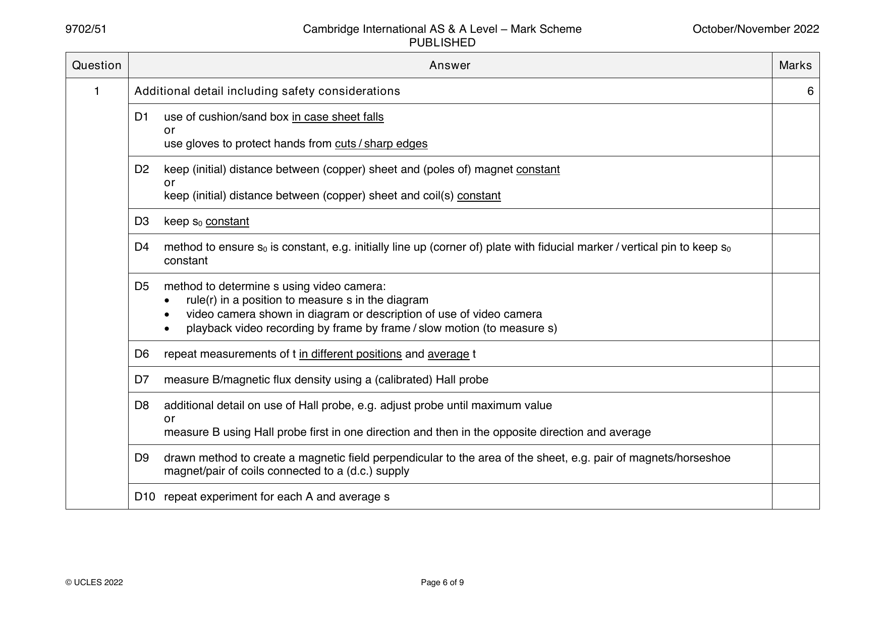
1 Additional detail including safety considerations 6
D1 use of cushion/sand box in case sheet falls
or
use gloves to protect hands from cuts / sharp edges
D2 keep (initial) distance between (copper) sheet and (poles of) magnet constant
or
keep (initial) distance between (copper) sheet and coil(s) constant
D3 keep s constant
0
D4 method to ensure s is constant, e.g. initially line up (corner of) plate with fiducial marker / vertical pin to keep s
0 0
constant
D5 method to determine s using video camera:
• rule(r) in a position to measure s in the diagram
• video camera shown in diagram or description of use of video camera
• playback video recording by frame by frame / slow motion (to measure s)
D6 repeat measurements of t in different positions and average t
D7 measure B/magnetic flux density using a (calibrated) Hall probe
D8 additional detail on use of Hall probe, e.g. adjust probe until maximum value
or
measure B using Hall probe first in one direction and then in the opposite direction and average
D9 drawn method to create a magnetic field perpendicular to the area of the sheet, e.g. pair of magnets/horseshoe
magnet/pair of coils connected to a (d.c.) supply
D10 repeat experiment for each A and average s
© UCLES 2022 Page 6 of 9
Official mark scheme pages: 5, 6 · source PDF URL
9702-2022-on-51-q02
Oct/Nov 2022 · Paper 51 · Question 2 · 15 marks
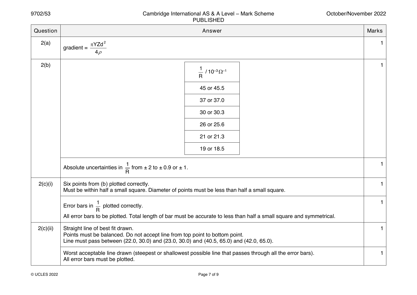
2(a) YZd2 1
gradient =
4
2(b) 1
1
/ 10–3 –1
R
45 or 45.5
37 or 37.0
30 or 30.3
26 or 25.6
21 or 21.3
19 or 18.5
1 1
Absolute uncertainties in from ± 2 to ± 0.9 or ± 1.
R
2(c)(i) Six points from (b) plotted correctly. 1
Must be within half a small square. Diameter of points must be less than half a small square.
1 1
Error bars in plotted correctly.
R
All error bars to be plotted. Total length of bar must be accurate to less than half a small square and symmetrical.
2(c)(ii) Straight line of best fit drawn. 1
Points must be balanced. Do not accept line from top point to bottom point.
Line must pass between (22.0, 30.0) and (23.0, 30.0) and (40.5, 65.0) and (42.0, 65.0).
Worst acceptable line drawn (steepest or shallowest possible line that passes through all the error bars). 1
All error bars must be plotted.
© UCLES 2022 Page 7 of 9
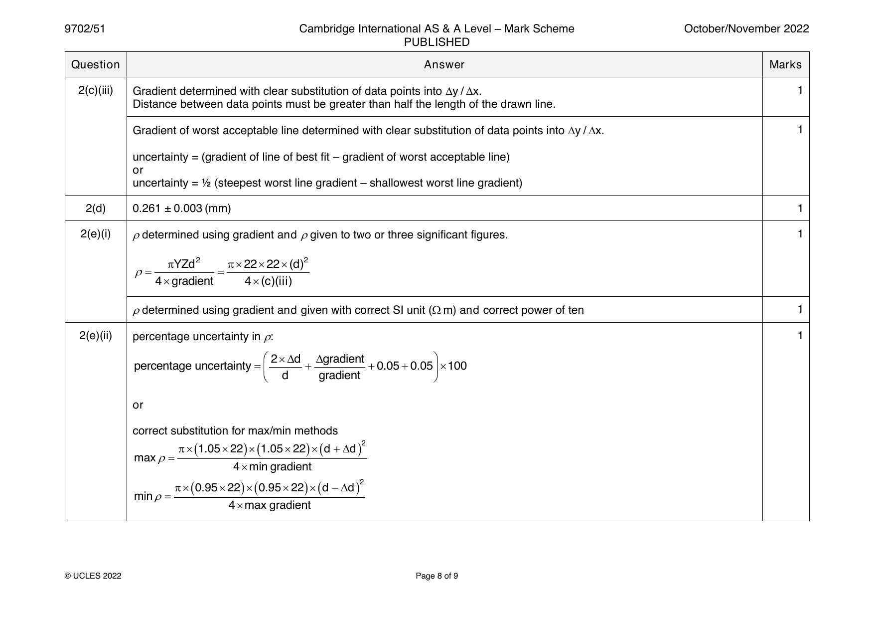
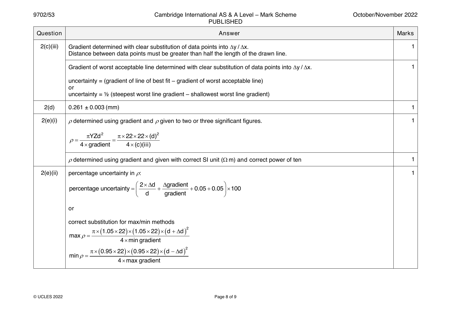
2(c)(iii) Gradient determined with clear substitution of data points into y / x. 1
Distance between data points must be greater than half the length of the drawn line.
Gradient of worst acceptable line determined with clear substitution of data points into y / x. 1
uncertainty = (gradient of line of best fit – gradient of worst acceptable line)
or
uncertainty = ½ (steepest worst line gradient – shallowest worst line gradient)
2(d) 0.261 ± 0.003 (mm) 1
2(e)(i) determined using gradient and given to two or three significant figures. 1
YZd2 2222(d)2
= =
4gradient 4(c)(iii)
determined using gradient and given with correct SI unit ( m) and correct power of ten 1
2(e)(ii) percentage uncertainty in : 1
2d gradient
percentage uncertainty= + +0.05+0.05100
d gradient
or
correct substitution for max/min methods
(1.0522)(1.0522)(d +d)2
max=
4mingradient
(0.9522)(0.9522)(d −d)2
min=
4maxgradient
© UCLES 2022 Page 8 of 9
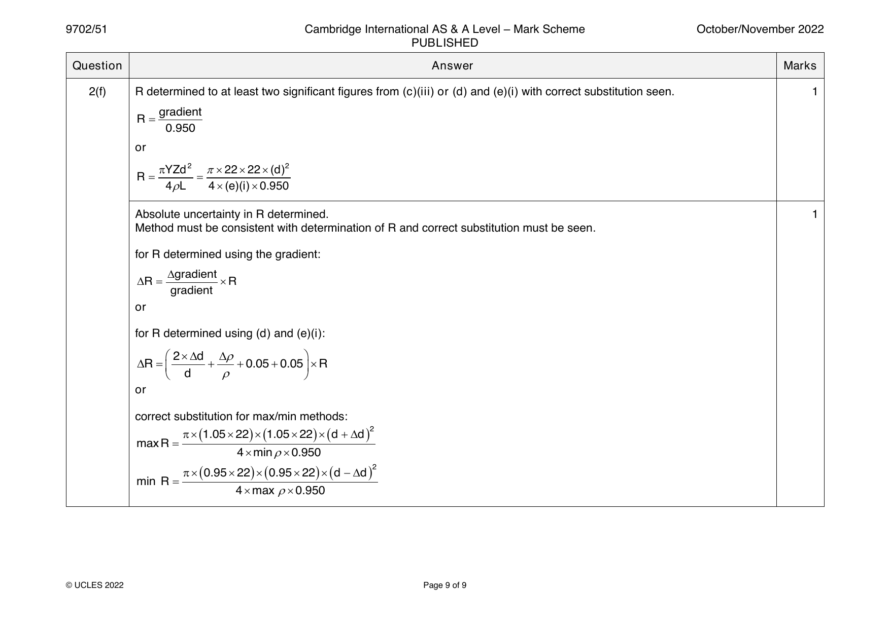
2(f) R determined to at least two significant figures from (c)(iii) or (d) and (e)(i) with correct substitution seen. 1
gradient
R =
0.950
or
YZd2 2222(d)2
R = =
4L 4(e)(i)0.950
Absolute uncertainty in R determined. 1
Method must be consistent with determination of R and correct substitution must be seen.
for R determined using the gradient:
gradient
R = R
gradient
or
for R determined using (d) and (e)(i):
2d
R= + +0.05+0.05 R
d
or
correct substitution for max/min methods:
(1.0522)(1.0522)(d +d)2
maxR =
4min0.950
(0.9522)(0.9522)(d −d)2
min R =
4max0.950
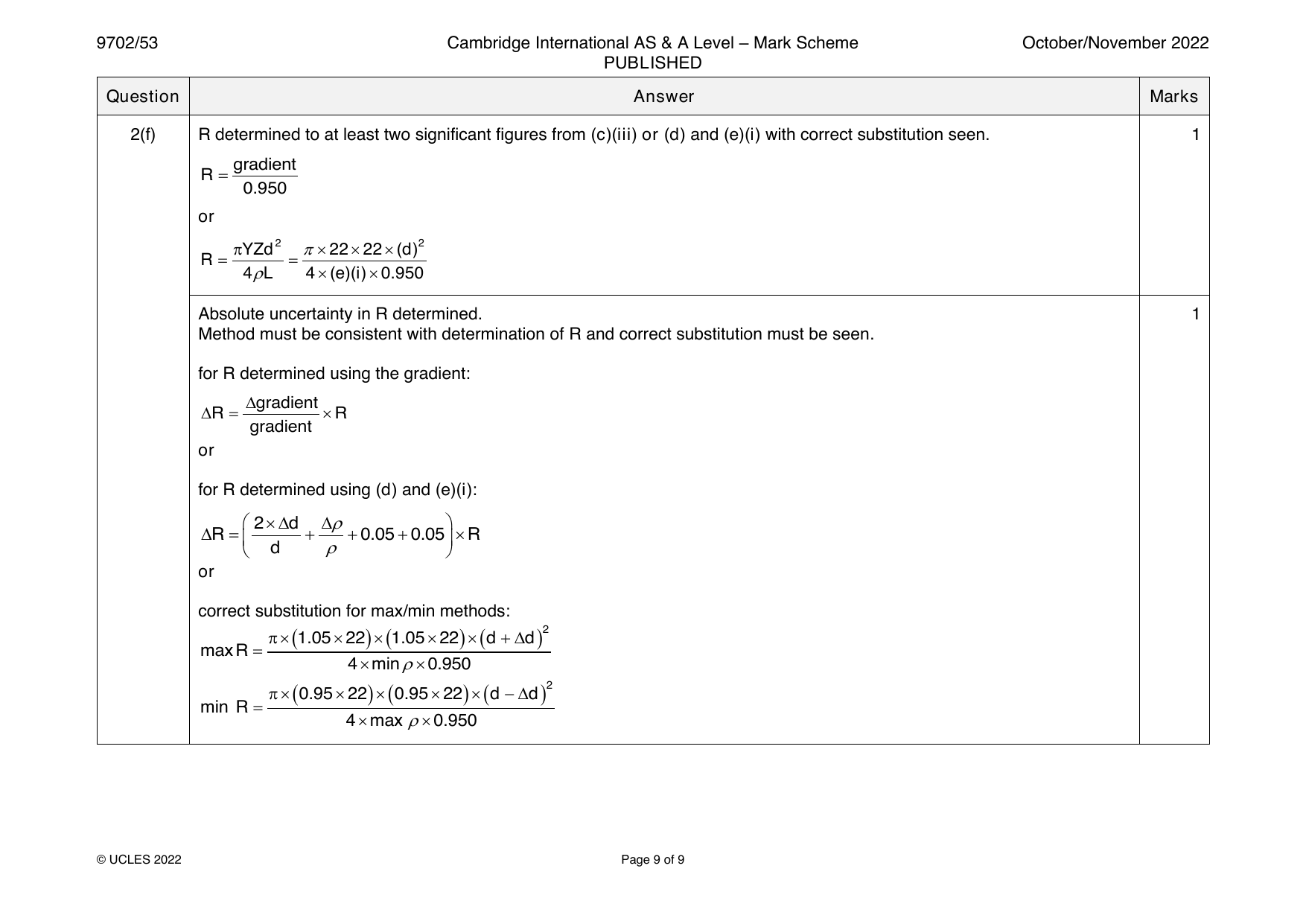
© UCLES 2022 Page 9 of 9
Official mark scheme pages: 7, 8, 9 · source PDF URL
9702-2022-on-52-q01
Oct/Nov 2022 · Paper 52 · Question 1 · 15 marks
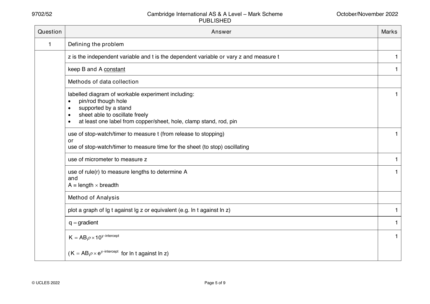
1 Defining the problem
z is the independent variable and t is the dependent variable or vary z and measure t 1
keep B and A constant 1
Methods of data collection
labelled diagram of workable experiment including: 1
• pin/rod though hole
• supported by a stand
• sheet able to oscillate freely
• at least one label from copper/sheet, hole, clamp stand, rod, pin
use of stop-watch/timer to measure t (from release to stopping) 1
or
use of stop-watch/timer to measure time for the sheet (to stop) oscillating
use of micrometer to measure z 1
use of rule(r) to measure lengths to determine A 1
and
A = length breadth
Method of Analysis
plot a graph of lg t against lg z or equivalent (e.g. ln t against ln z) 1
q=gradient 1
K = AB10y-intercept 1
(K = ABey-intercept for ln t against ln z)
© UCLES 2022 Page 5 of 9
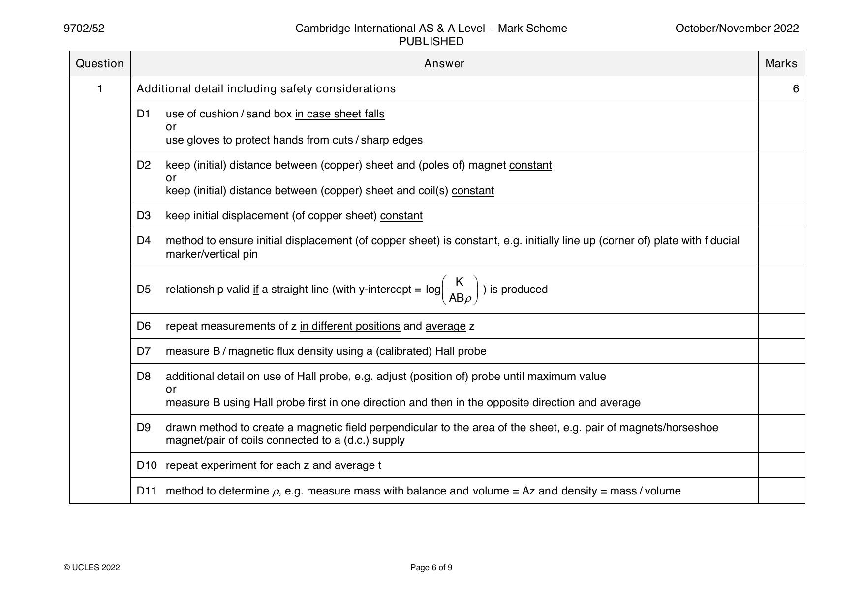
1 Additional detail including safety considerations 6
D1 use of cushion / sand box in case sheet falls
or
use gloves to protect hands from cuts / sharp edges
D2 keep (initial) distance between (copper) sheet and (poles of) magnet constant
or
keep (initial) distance between (copper) sheet and coil(s) constant
D3 keep initial displacement (of copper sheet) constant
D4 method to ensure initial displacement (of copper sheet) is constant, e.g. initially line up (corner of) plate with fiducial
marker/vertical pin
K
D5 relationship valid if a straight line (with y-intercept = log ) is produced
AB
D6 repeat measurements of z in different positions and average z
D7 measure B / magnetic flux density using a (calibrated) Hall probe
D8 additional detail on use of Hall probe, e.g. adjust (position of) probe until maximum value
or
measure B using Hall probe first in one direction and then in the opposite direction and average
D9 drawn method to create a magnetic field perpendicular to the area of the sheet, e.g. pair of magnets/horseshoe
magnet/pair of coils connected to a (d.c.) supply
D10 repeat experiment for each z and average t
D11 method to determine , e.g. measure mass with balance and volume = Az and density = mass / volume
© UCLES 2022 Page 6 of 9
Official mark scheme pages: 5, 6 · source PDF URL
9702-2022-on-52-q02
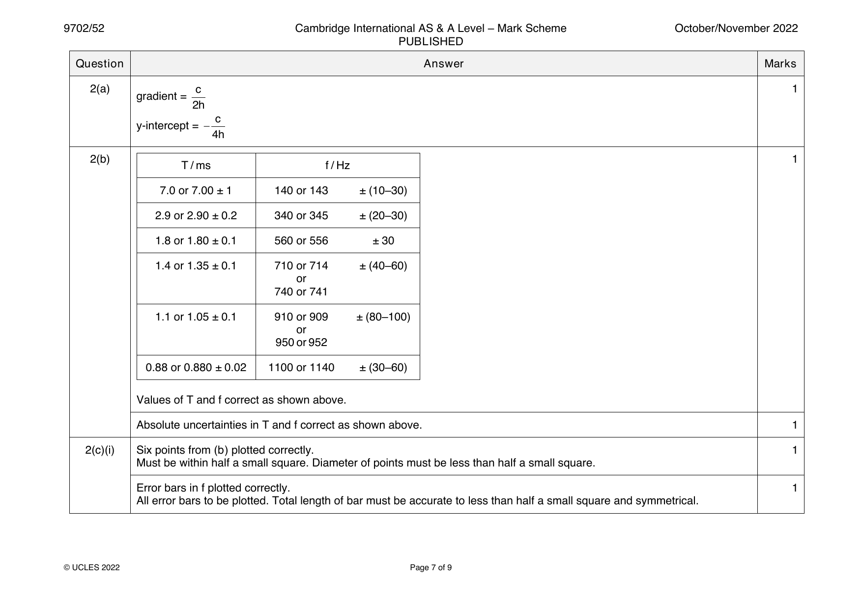
Oct/Nov 2022 · Paper 52 · Question 2 · 15 marks
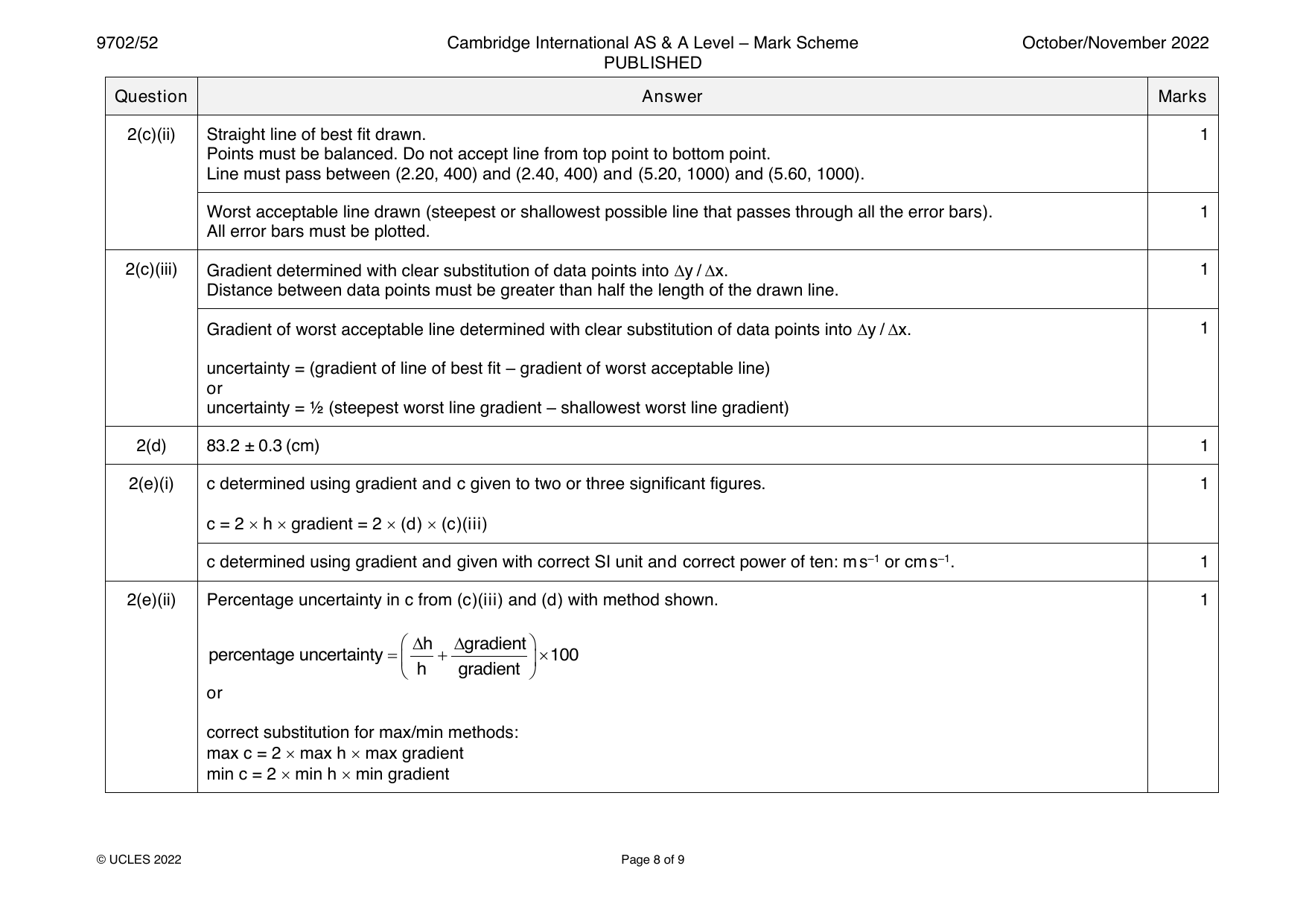
2(a) c 1
gradient =
2h
c
y-intercept = −
4h
2(b) 1
T / ms f / Hz
7.0 or 7.00 ± 1 140 or 143 ± (10–30)
2.9 or 2.90 ± 0.2 340 or 345 ± (20–30)
1.8 or 1.80 ± 0.1 560 or 556 ± 30
1.4 or 1.35 ± 0.1 710 or 714 ± (40–60)
or
740 or 741
1.1 or 1.05 ± 0.1 910 or 909 ± (80–100)
or
950or952
0.88 or 0.880 ± 0.02 1100 or 1140 ± (30–60)
Values of T and f correct as shown above.
Absolute uncertainties in T and f correct as shown above. 1
2(c)(i) Six points from (b) plotted correctly. 1
Must be within half a small square. Diameter of points must be less than half a small square.
Error bars in f plotted correctly. 1
All error bars to be plotted. Total length of bar must be accurate to less than half a small square and symmetrical.
© UCLES 2022 Page 7 of 9
2(c)(ii) Straight line of best fit drawn. 1
Points must be balanced. Do not accept line from top point to bottom point.
Line must pass between (2.20, 400) and (2.40, 400) and (5.20, 1000) and (5.60, 1000).
Worst acceptable line drawn (steepest or shallowest possible line that passes through all the error bars). 1
All error bars must be plotted.
2(c)(iii) Gradient determined with clear substitution of data points into y / x. 1
Distance between data points must be greater than half the length of the drawn line.
Gradient of worst acceptable line determined with clear substitution of data points into y / x. 1
uncertainty = (gradient of line of best fit – gradient of worst acceptable line)
or
uncertainty = ½ (steepest worst line gradient – shallowest worst line gradient)
2(d) 83.2 ± 0.3 (cm) 1
2(e)(i) c determined using gradient and c given to two or three significant figures. 1
c = 2 h gradient = 2 (d) (c)(iii)
c determined using gradient and given with correct SI unit and correct power of ten: m s–1 or cm s–1. 1
2(e)(ii) Percentage uncertainty in c from (c)(iii) and (d) with method shown. 1
h gradient
percentage uncertainty= + 100
h gradient
or
correct substitution for max/min methods:
max c = 2 max h max gradient
min c = 2 min h min gradient
© UCLES 2022 Page 8 of 9
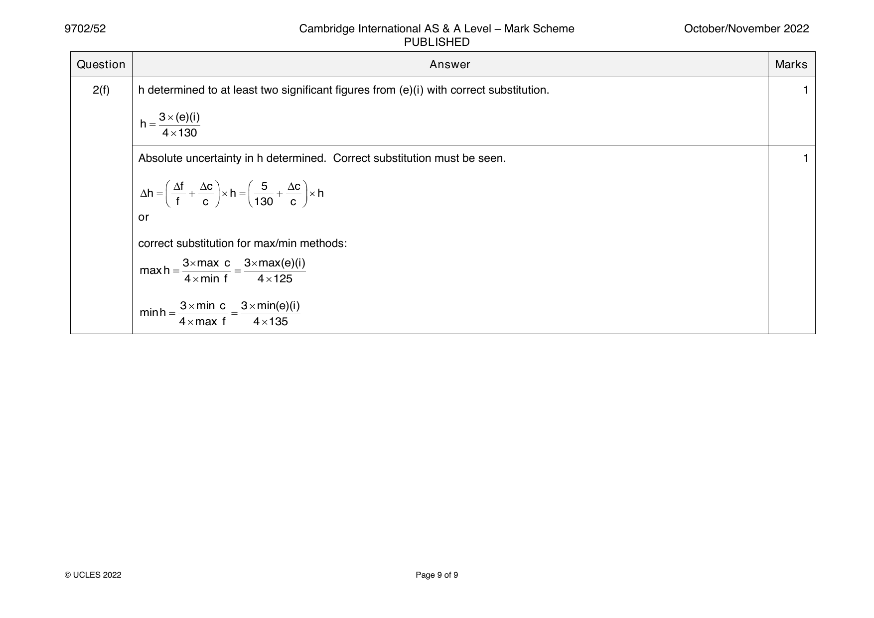
2(f) h determined to at least two significant figures from (e)(i) with correct substitution. 1
3(e)(i)
h=
4130
Absolute uncertainty in h determined. Correct substitution must be seen. 1
f c 5 c
h= + h= + h
f c 130 c
or
correct substitution for max/min methods:
3 max c 3 max(e)(i)
maxh= =
4min f 4125
3min c 3min(e)(i)
minh= =
4max f 4135
© UCLES 2022 Page 9 of 9
Official mark scheme pages: 7, 8, 9 · source PDF URL
9702-2022-on-53-q01
Oct/Nov 2022 · Paper 53 · Question 1 · 15 marks
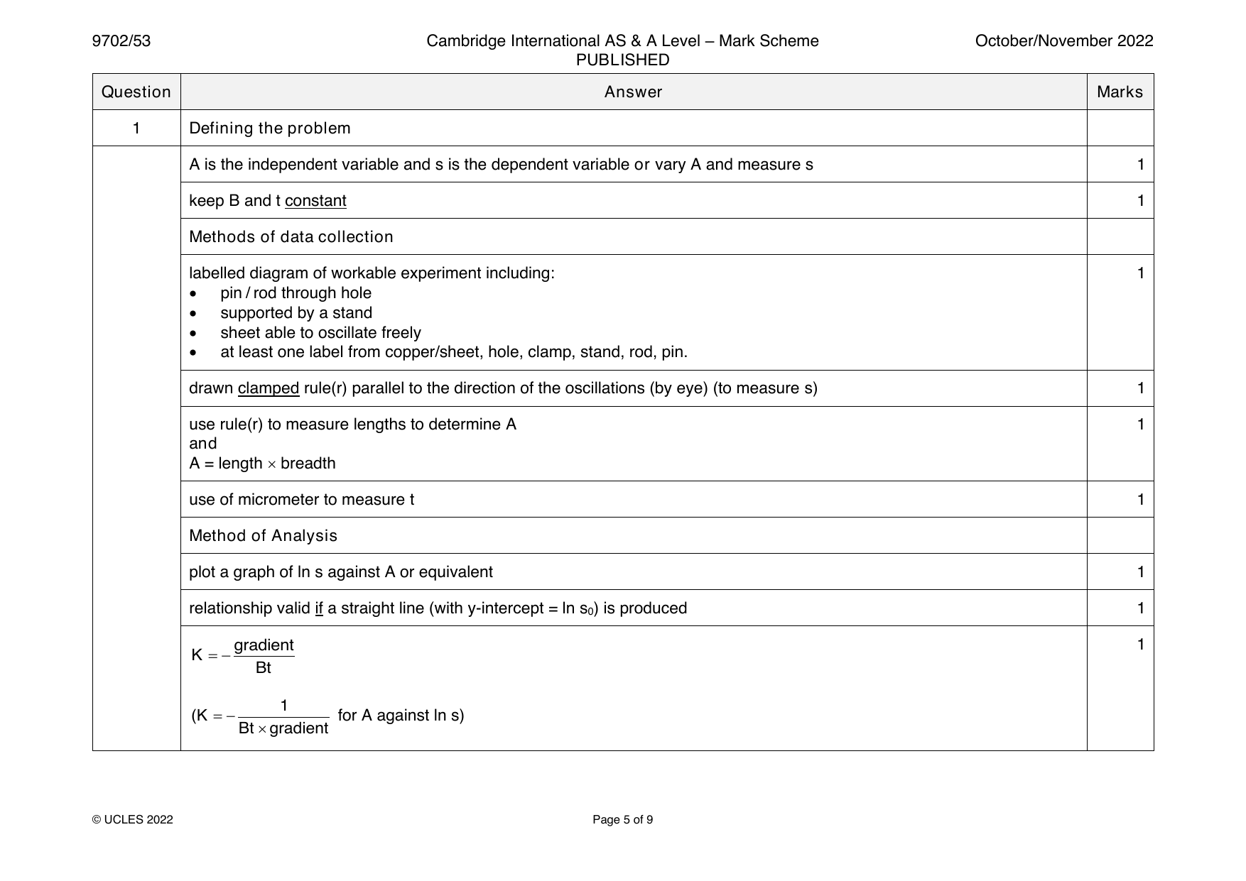
1 Defining the problem
A is the independent variable and s is the dependent variable or vary A and measure s 1
keep B and t constant 1
Methods of data collection
labelled diagram of workable experiment including: 1
• pin / rod through hole
• supported by a stand
• sheet able to oscillate freely
• at least one label from copper/sheet, hole, clamp, stand, rod, pin.
drawn clamped rule(r) parallel to the direction of the oscillations (by eye) (to measure s) 1
use rule(r) to measure lengths to determine A 1
and
A = length breadth
use of micrometer to measure t 1
Method of Analysis
plot a graph of ln s against A or equivalent 1
relationship valid if a straight line (with y-intercept = ln s ) is produced 1
0
gradient 1
K =−
Bt
1
(K =− for A against ln s)
Btgradient
© UCLES 2022 Page 5 of 9
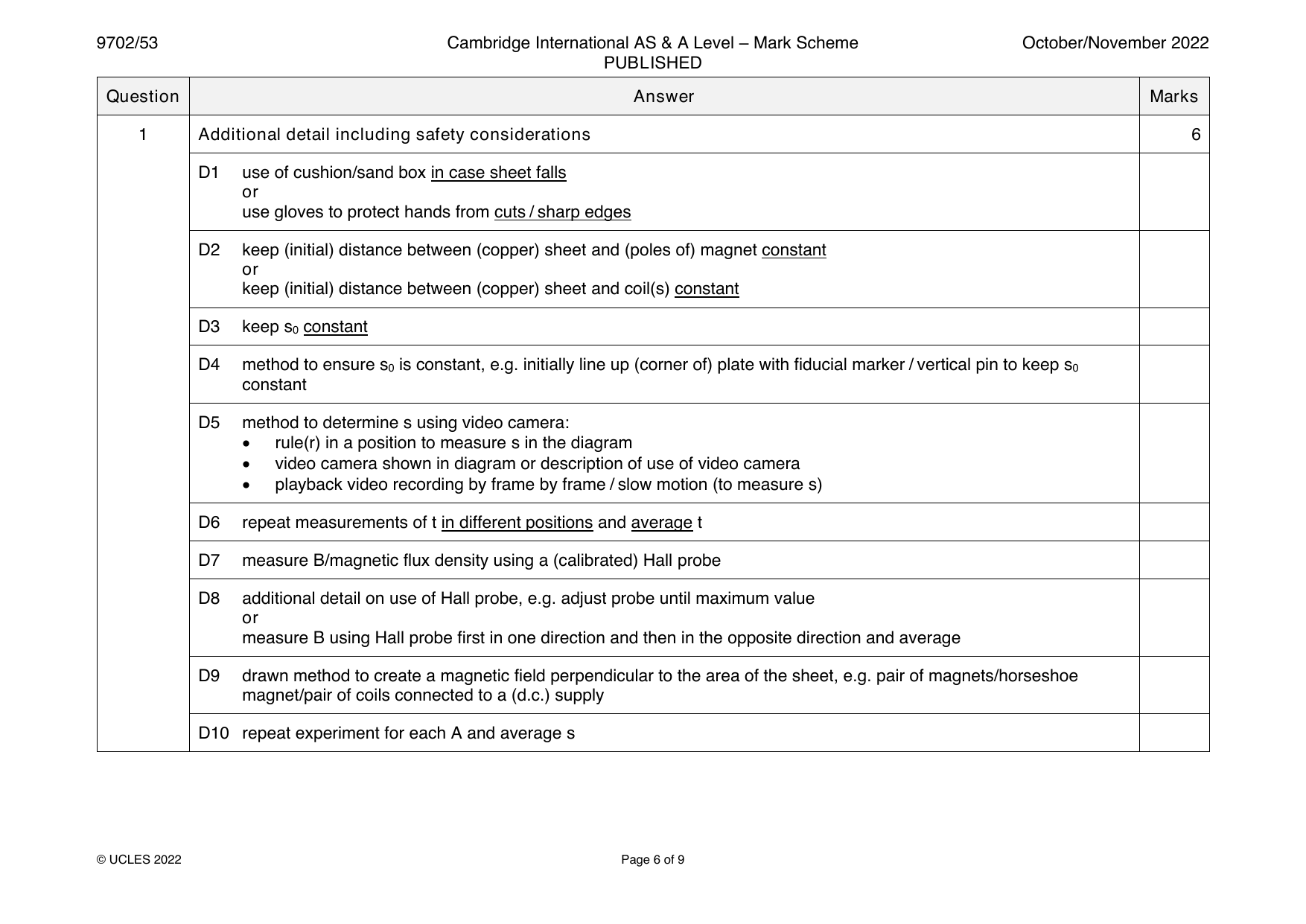
1 Additional detail including safety considerations 6
D1 use of cushion/sand box in case sheet falls
or
use gloves to protect hands from cuts / sharp edges
D2 keep (initial) distance between (copper) sheet and (poles of) magnet constant
or
keep (initial) distance between (copper) sheet and coil(s) constant
D3 keep s constant
0
D4 method to ensure s is constant, e.g. initially line up (corner of) plate with fiducial marker / vertical pin to keep s
0 0
constant
D5 method to determine s using video camera:
• rule(r) in a position to measure s in the diagram
• video camera shown in diagram or description of use of video camera
• playback video recording by frame by frame / slow motion (to measure s)
D6 repeat measurements of t in different positions and average t
D7 measure B/magnetic flux density using a (calibrated) Hall probe
D8 additional detail on use of Hall probe, e.g. adjust probe until maximum value
or
measure B using Hall probe first in one direction and then in the opposite direction and average
D9 drawn method to create a magnetic field perpendicular to the area of the sheet, e.g. pair of magnets/horseshoe
magnet/pair of coils connected to a (d.c.) supply
D10 repeat experiment for each A and average s
© UCLES 2022 Page 6 of 9
Official mark scheme pages: 5, 6 · source PDF URL
9702-2022-on-53-q02
Oct/Nov 2022 · Paper 53 · Question 2 · 15 marks
2(a) YZd2 1
gradient =
4
2(b) 1
1
/ 10–3 –1
R
45 or 45.5
37 or 37.0
30 or 30.3
26 or 25.6
21 or 21.3
19 or 18.5
1 1
Absolute uncertainties in from ± 2 to ± 0.9 or ± 1.
R
2(c)(i) Six points from (b) plotted correctly. 1
Must be within half a small square. Diameter of points must be less than half a small square.
1 1
Error bars in plotted correctly.
R
All error bars to be plotted. Total length of bar must be accurate to less than half a small square and symmetrical.
2(c)(ii) Straight line of best fit drawn. 1
Points must be balanced. Do not accept line from top point to bottom point.
Line must pass between (22.0, 30.0) and (23.0, 30.0) and (40.5, 65.0) and (42.0, 65.0).
Worst acceptable line drawn (steepest or shallowest possible line that passes through all the error bars). 1
All error bars must be plotted.
© UCLES 2022 Page 7 of 9
2(c)(iii) Gradient determined with clear substitution of data points into y / x. 1
Distance between data points must be greater than half the length of the drawn line.
Gradient of worst acceptable line determined with clear substitution of data points into y / x. 1
uncertainty = (gradient of line of best fit – gradient of worst acceptable line)
or
uncertainty = ½ (steepest worst line gradient – shallowest worst line gradient)
2(d) 0.261 ± 0.003 (mm) 1
2(e)(i) determined using gradient and given to two or three significant figures. 1
YZd2 2222(d)2
= =
4gradient 4(c)(iii)
determined using gradient and given with correct SI unit ( m) and correct power of ten 1
2(e)(ii) percentage uncertainty in : 1
2d gradient
percentage uncertainty= + +0.05+0.05100
d gradient
or
correct substitution for max/min methods
(1.0522)(1.0522)(d +d)2
max=
4mingradient
(0.9522)(0.9522)(d −d)2
min=
4maxgradient
© UCLES 2022 Page 8 of 9
2(f) R determined to at least two significant figures from (c)(iii) or (d) and (e)(i) with correct substitution seen. 1
gradient
R =
0.950
or
YZd2 2222(d)2
R = =
4L 4(e)(i)0.950
Absolute uncertainty in R determined. 1
Method must be consistent with determination of R and correct substitution must be seen.
for R determined using the gradient:
gradient
R = R
gradient
or
for R determined using (d) and (e)(i):
2d
R= + +0.05+0.05 R
d
or
correct substitution for max/min methods:
(1.0522)(1.0522)(d +d)2
maxR =
4min0.950
(0.9522)(0.9522)(d −d)2
min R =
4max0.950
© UCLES 2022 Page 9 of 9
Official mark scheme pages: 7, 8, 9 · source PDF URL
9702-2023-m-52-q01
March 2023 · Paper 52 · Question 1 · 15 marks
1 Defining the problem
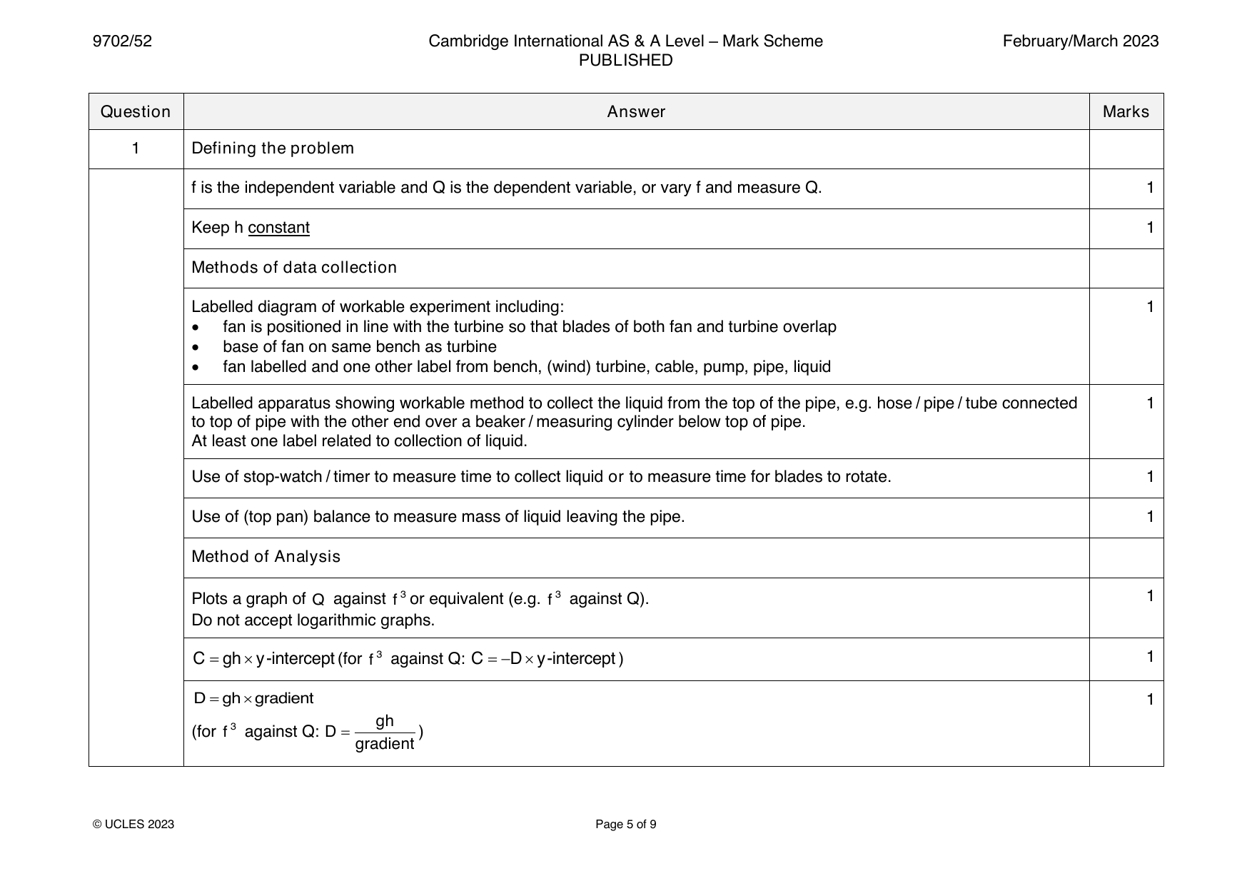
f is the independent variable and Q is the dependent variable, or vary f and measure Q. 1
Keep h constant 1
Methods of data collection
Labelled diagram of workable experiment including: 1
• fan is positioned in line with the turbine so that blades of both fan and turbine overlap
• base of fan on same bench as turbine
• fan labelled and one other label from bench, (wind) turbine, cable, pump, pipe, liquid
Labelled apparatus showing workable method to collect the liquid from the top of the pipe, e.g. hose / pipe / tube connected 1
to top of pipe with the other end over a beaker / measuring cylinder below top of pipe.
At least one label related to collection of liquid.
Use of stop-watch / timer to measure time to collect liquid or to measure time for blades to rotate. 1
Use of (top pan) balance to measure mass of liquid leaving the pipe. 1
Method of Analysis
Plots a graph of Q against f3or equivalent (e.g. f3 against Q). 1
Do not accept logarithmic graphs.
C =ghy-intercept(for f3 against Q: C =−Dy-intercept) 1
D=ghgradient 1
gh
(for f3 against Q: D = )
gradient
© UCLES 2023 Page 5 of 9
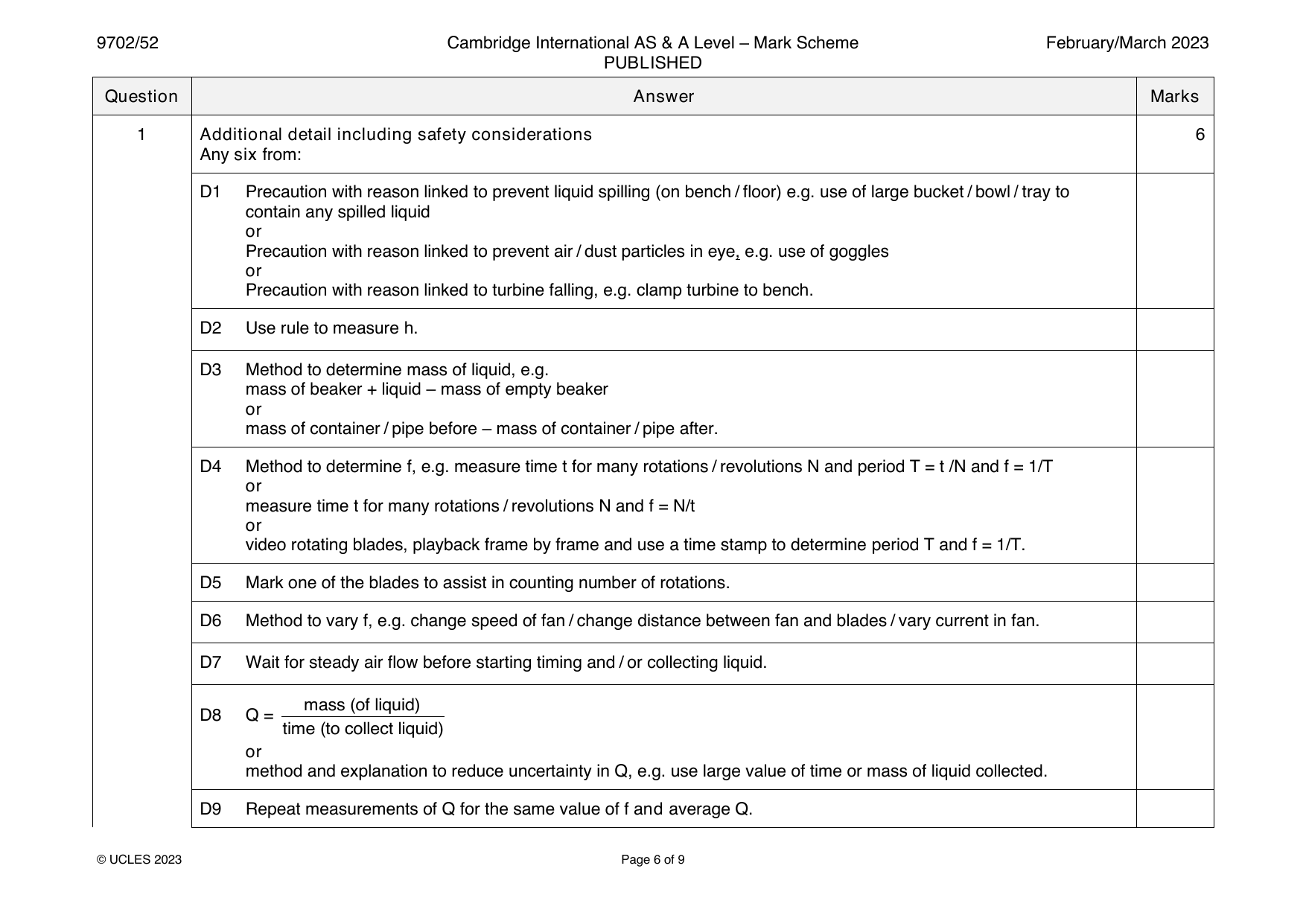
1 Additional detail including safety considerations 6
Any six from:
D1 Precaution with reason linked to prevent liquid spilling (on bench / floor) e.g. use of large bucket / bowl / tray to
contain any spilled liquid
or
Precaution with reason linked to prevent air / dust particles in eye, e.g. use of goggles
or
Precaution with reason linked to turbine falling, e.g. clamp turbine to bench.
D2 Use rule to measure h.
D3 Method to determine mass of liquid, e.g.
mass of beaker + liquid – mass of empty beaker
or
mass of container / pipe before – mass of container / pipe after.
D4 Method to determine f, e.g. measure time t for many rotations / revolutions N and period T = t /N and f = 1/T
or
measure time t for many rotations / revolutions N and f = N/t
or
video rotating blades, playback frame by frame and use a time stamp to determine period T and f = 1/T.
D5 Mark one of the blades to assist in counting number of rotations.
D6 Method to vary f, e.g. change speed of fan / change distance between fan and blades / vary current in fan.
D7 Wait for steady air flow before starting timing and / or collecting liquid.
mass (of liquid)
D8 Q =
time (to collect liquid)
or
method and explanation to reduce uncertainty in Q, e.g. use large value of time or mass of liquid collected.
D9 Repeat measurements of Q for the same value of f and average Q.
© UCLES 2023 Page 6 of 9
1 D10 Relationship valid if a straight line is produced (not passing through the origin).
Do not accept passing through the origin.
Question Answer Marks
Official mark scheme pages: 5, 6, 7 · source PDF URL
9702-2023-m-52-q02
March 2023 · Paper 52 · Question 2 · 15 marks
2(a) v 1
gradient =
4
y-intercept = −k
2(b) 2
1/f / 10–3 Hz–1 d / cm
0.67 or 0.667 24.7 0.2
0.48 or 0.476 17.4 0.2
0.36 or 0.357 12.7 0.3
0.24 or 0.244 8.4 0.3
0.19 or 0.192 6.6 0.4
0.13 or 0.132 4.6 0.4
First mark: values of 1 / f and d correct as shown.
Second mark: uncertainties in d correct as shown.
2(c)(i) Six points from (b) plotted correctly. 1
Must be within half a small square. Diameter of points must be less than half a small square.
Error bars in d / cm plotted correctly. 1
All error bars to be plotted. Total length of bar must be accurate to less than half a small square and symmetrical.
© UCLES 2023 Page 7 of 9
2(c)(ii) Straight line of best fit drawn. 1
Do not accept line from top plot to bottom plot.
Points must be balanced.
Line must pass between (0.170, 6.0) and (0.185, 6.0) and between (0.590, 22.0) and (0.610, 22.0)
Worst acceptable line drawn. 1
Steepest or shallowest possible line that passes through all the error bars.
All error bars must be plotted.
2(c)(iii) Gradient determined with clear substitution of data points into y / x; distance between data points must be greater than 1
half the length of the drawn line.
Gradient determined of worst acceptable line uncertainty = (gradient of line of best fit – gradient of worst acceptable line) 1
or
uncertainty = ½ (steepest worst line gradient – shallowest worst line gradient)
2(c)(iv) y-intercept determined by substitution of correct point with consistent power of ten in m and x into y = mx + c. 1
Expect y-intercept to be negative.
y-intercept of worst acceptable line determined by substitution into y = mx + c. 1
uncertainty = y-intercept of line of best fit – y-intercept of worst acceptable line, or
uncertainty = ½ (steepest worst line y-intercept – shallowest worst line y-intercept)
© UCLES 2023 Page 8 of 9
2(d) v determined using gradient and v and k given to 2 or 3 sf. 1
v =4gradient=4(c)(iii)
k determined using y-intercept and units for v and k 1
k =−y-intercept=−(c)(iv)
Units:
v: m s–1, cm s–1
k: m, cm
Absolute uncertainties in v and k. 1
gradient
v: v with correct substitution or v: 4 uncertainty in gradient
gradient
and
k: uncertainty in y-intercept
2(e) f determined to a minimum of 2 significant figures from (c)(iii) and (c)(iv) OR (d) with correct substitution and correct 1
powers of ten used for all quantities.
v
f =
4(d +k)
or
gradient
f =
d −(y-intercept)
© UCLES 2023 Page 9 of 9
Official mark scheme pages: 7, 8, 9 · source PDF URL
9702-2023-mj-51-q01
May/June 2023 · Paper 51 · Question 1 · 15 marks
1 Defining the problem
is the independent variable and t is the dependent variable or vary and measure t 1
keep d constant 1
Methods of data collection
labelled diagram of workable experiment including: 1
plane supported by stand / support
stand/support on bench/floor/horizontal surface
minimum of two labels from cube, cylinder, (inclined) plane, method of support, bench/floor/horizontal surface, pulley,
string
diagram showing method to measure d, e.g. 1
clamped vertical rule near cylinder
or
drawn rule on plane used to measure d
or
distance d marked on plane and rule used to determine d
use a protractor to measure θ 1
or
use a rule(r) to measure appropriate lengths for a trigonometric calculation
use a timer/stop-watch to measure t or light gates connected to a timer to measure t 1
© UCLES 2023 Page 6 of 12
1 Method of Analysis
1 1 1
plot a graph of against sin or equivalent (e.g. sin against )
t2 t2
Do not accept logarithms.
2dABgradient 1
H
A
1
2dAB
(for sin against : H )
t2 Agradient
2dABy-intercept 1
K
A
1
(for sin against : K Hy-intercept)
t2
© UCLES 2023 Page 7 of 12
1 Additional detail including safety considerations 6
D1 Safety precaution linked to falling cylinder, e.g. use of cushion/sand box to collect cylinder/prevent damage to
cylinder/floor/bench/injury
D2 protractor correctly positioned on diagram
or
appropriate trigonometric relationship for marked lengths
D3 keep A and B constant
D4 use a (top-pan) balance to measure A and B
D5 correct positioning of light gates to determine t, e.g. two light gates either end of distance d, connected to a timer
or
correct position of video camera with timer in frame of the video to determine t
D6 method to release cylinder/cube, e.g. cube held by set square, set square moved to release cube.
D7 reasoned method to keep d constant as θ changes, e.g.
(when measuring d by position of cylinder) adjust the length of the string or adjust the position of vertical marks or
adjust the position of the vertical rule or initial position of the cube
or
(when measuring d by position of cube) use fixed marks on the plane or ruler placed on the plane with d measured
between the marks
D8 method to increase t for cylinder to fall, e.g. use large d to increase t
D9 repeat measurements of t for the same θ and average t
D10 relationship valid if a straight line is produced (not passing through the origin)
Do not accept straight line passing through the origin.
© UCLES 2023 Page 8 of 12
Official mark scheme pages: 6, 7, 8 · source PDF URL
9702-2023-mj-51-q02
May/June 2023 · Paper 51 · Question 2 · 15 marks
2(a) V 1
gradient = Rln
V
0
2(b) 1
C / 10–4 F T / s
0.89 or 0.892 13.7 0.8
1.3 or 1.32 20.4 0.7
1.6 or 1.58 24.3 0.6
1.0 or 1.03 16.1 0.8
1.2 or 1.18 18.3 0.7
2.1 or 2.08 31.5 0.6
Values of C and T correct as shown above.
Absolute uncertainties in T correct as shown above. 1
2(c)(i) Six points from (b) plotted correctly. 1
Must be within half a small square. Diameter of points must be less than half a small square.
Error bars in T plotted correctly. 1
All error bars to be plotted. Total length of bar must be accurate to less than half a small square and symmetrical.
© UCLES 2023 Page 9 of 12
2(c)(ii) Straight line of best fit drawn. 1
Do not accept line from top point to bottom point.
Points must be balanced.
Line must pass between (1.42, 22.0) and (1.45, 22.0) and between (1.95, 30.0) and (2.00, 30.0)
Worst acceptable line drawn (steepest or shallowest possible line that passes through all the error bars). 1
All error bars must be plotted.
2(c)(iii) Gradient determined with clear substitution of data points into y / x. 1
Distance between data points must be greater than half the length of the drawn line.
Gradient of worst acceptable line determined with clear substitution of data points into y / x. 1
uncertainty = (gradient of line of best fit – gradient of worst acceptable line)
or
uncertainty = ½ (steepest worst line gradient – shallowest worst line gradient)
2(d) – 0.69 or – 0.693 and 0.06 1
2(e)(i) R determined using gradient and R given to 2 or 3 significant figures. 1
gradient (c)(iii)
R
V (d)
ln
V
0
R correctly determined using gradient and SI unit with correct power of ten for R (e.g. ). 1
© UCLES 2023 Page 10 of 12
2(e)(ii) Percentage uncertainty in R with method shown. 1
V
ln
percentage uncertainty V 0 gradient 100
V gradient
ln
V
0
or
Correct substitution for max/min methods.
© UCLES 2023 Page 11 of 12
2(f) C determined to a minimum of 2 significant figures from (c)(iii) or (d) and (e)(i) with correct substitution. 1
T 60.0
C
gradient gradient
or
T 60.0
C
V (e)(i)(d)
Rln
V
0
Absolute uncertainty in C determined with correct method used: 1
Using gradient to determine C:
gradient
C C
gradient
Allow using R to determine C:
V
ln
C V 0 (e)(ii) C
V 100
ln
V
0
© UCLES 2023 Page 12 of 12
Official mark scheme pages: 9, 10, 11, 12 · source PDF URL
9702-2023-mj-52-q01
May/June 2023 · Paper 52 · Question 1 · 15 marks
1 Defining the problem
R is the independent variable and E is the dependent variable or vary R and measure E 1
keep V constant 1
Methods of data collection
labelled diagram of workable experiment including: 1
coil P placed close to coil Q
separate workable circuit for coil Q
(a.c.) voltmeter or oscilloscope connected across coil Q
(Do not accept a power supply connected to coil Q.)
a.c. power supply/signal generator connected to resistor and coil P in series 1
workable circuit with power supply and (a.c.) voltmeter/oscilloscope in parallel with resistor and coil P or across terminals of 1
power supply/signal generator
method to determine R, e.g. measure current in R and p.d. across R and use R = V /I or measure R using an ohmmeter 1
R
© UCLES 2023 Page 6 of 12
1 Method of Analysis
1 1 1
plot a graph of against R or equivalent (e.g. R against )
E E
Do not accept logarithms.
1 1
M
2fV gradient
1 gradient
(for R against : M )
E 2fV
k 2fVMy-intercept 1
or
y-intercept
k
gradient
1
(for R against : k = y-intercept)
E
© UCLES 2023 Page 7 of 12
1 Additional detail including safety considerations 6
D1 precaution linked to hot coil (P) / hot resistor, e.g. use of (heat-proof) gloves, wait until circuit cools down
or
precaution linked to shocks from high voltages e.g. use of (insulating) gloves or switch off supply before touching the
circuit (to change R)
D2 keep the number of turns on (both) coils constant
D3 keep f constant
D4 keep distance between the coils constant
D5 method to keep distance between the coils constant, e.g. fix/clamp coils to bench
D6 method to measure f, e.g. read from signal generator or use of oscilloscope
D7 method to determine f from oscilloscope, e.g. period from oscilloscope T = time-base horizontal distance and
f = 1/T
D8 method to determine V or E from oscilloscope, e.g. V = y-gain vertical distance
D9 method to increase E e.g. use iron core/more turns on coil Q/high frequency/high p.d. (across R and coil P)
D10 relationship valid if a straight line is produced (not passing through the origin)
Do not accept straight line passing through the origin.
© UCLES 2023 Page 8 of 12
Official mark scheme pages: 6, 7, 8 · source PDF URL
9702-2023-mj-52-q02
May/June 2023 · Paper 52 · Question 2 · 15 marks
2(a) Yk 1
gradient =
p
YkZ
y-intercept =
p
2(b) 1
V / 10–5 m3 absolute uncertainty
3.81 or 3.815 0.03
3.99 or 3.986 0.03
4.16 or 4.163 0.04
4.33 or 4.335 0.04
4.48 or 4.481 0.04
4.65 or 4.652 0.04
Values of V correct as shown above.
Absolute uncertainties in V correct as shown above. 1
2(c)(i) Six points from (b) plotted correctly. 1
Must be within half a small square. Diameter of points must be less than half a small square.
Error bars in V plotted correctly. 1
All error bars to be plotted. Total length of bar must be accurate to less than half a small square and symmetrical.
© UCLES 2023 Page 9 of 12
2(c)(ii) Straight line of best fit drawn. 1
Do not accept line from top point to bottom point.
Points must be balanced.
Line must pass between (27.5, 3.90) and (29.5, 3.90) and between (82.0, 4.60) and (84.0, 4.60).
Worst acceptable line drawn (steepest or shallowest possible line that passes through all the error bars). 1
All error bars must be plotted.
2(c)(iii) Gradient determined with clear substitution of data points into y / x. 1
Distance between data points must be greater than half the length of the drawn line.
Gradient of worst acceptable line determined with clear substitution of data points into y / x. 1
uncertainty = (gradient of line of best fit – gradient of worst acceptable line)
or
uncertainty = ½ (steepest worst line gradient – shallowest worst line gradient)
2(c)(iv) y-intercept determined by substitution of correct point with consistent power of ten in m and y into y = mx + c. 1
y-intercept of worst acceptable line determined by substitution into y = mx + c. 1
uncertainty = y-intercept of line of best fit – y-intercept of worst acceptable line
or
uncertainty = ½ (steepest worst line y-intercept – shallowest worst line y-intercept)
Do not accept ECF from false origin method.
© UCLES 2023 Page 10 of 12
2(d)(i) Y determined using gradient and Y and Z given to 2 or 3 significant figures. 1
pgradient
Y 7.31881027 gradient
k
Z determined using y-intercept and Y and Z given with SI units. 1
py-intercept y-intercept
Z or Z
Yk gradient
Units:
Y: no unit
Z: °C
2(d)(ii) Percentage uncertainty in Y with method shown. 1
p gradient
percentage uncertainty 100
p gradient
or
Correct substitution for max/min methods.
© UCLES 2023 Page 11 of 12
2(e) determined to a minimum of 2 significant figures from (c)(iii) and (c)(iv) or (d)(i) with correct substitution and correct 1
powers of ten.
0.02792
0.0600
V 3.67105
4
and
pV V V y-intercept
Z or Z or
Yk gradient gradient
or using h directly:
d2h
y-intercept
pd2h d2h
4
Z or Z or
4Yk 4gradient gradient
© UCLES 2023 Page 12 of 12
Official mark scheme pages: 9, 10, 11, 12 · source PDF URL
9702-2023-mj-53-q01
May/June 2023 · Paper 53 · Question 1 · 15 marks
1 Defining the problem
is the independent variable and t is the dependent variable or vary and measure t 1
keep d constant 1
Methods of data collection
labelled diagram of workable experiment including: 1
plane supported by stand / support
stand/support on bench/floor/horizontal surface
minimum of two labels from cube, cylinder, (inclined) plane, method of support, bench/floor/horizontal surface, pulley,
string
diagram showing method to measure d, e.g. 1
clamped vertical rule near cylinder
or
drawn rule on plane used to measure d
or
distance d marked on plane and rule used to determine d
use a protractor to measure θ 1
or
use a rule(r) to measure appropriate lengths for a trigonometric calculation
use a timer/stop-watch to measure t or light gates connected to a timer to measure t 1
© UCLES 2023 Page 6 of 12
1 Method of Analysis
1 1 1
plot a graph of against sin or equivalent (e.g. sin against )
t2 t2
Do not accept logarithms.
2dABgradient 1
H
A
1
2dAB
(for sin against : H )
t2 Agradient
2dABy-intercept 1
K
A
1
(for sin against : K Hy-intercept)
t2
© UCLES 2023 Page 7 of 12
1 Additional detail including safety considerations 6
D1 Safety precaution linked to falling cylinder, e.g. use of cushion/sand box to collect cylinder/prevent damage to
cylinder/floor/bench/injury
D2 protractor correctly positioned on diagram
or
appropriate trigonometric relationship for marked lengths
D3 keep A and B constant
D4 use a (top-pan) balance to measure A and B
D5 correct positioning of light gates to determine t, e.g. two light gates either end of distance d, connected to a timer
or
correct position of video camera with timer in frame of the video to determine t
D6 method to release cylinder/cube, e.g. cube held by set square, set square moved to release cube.
D7 reasoned method to keep d constant as θ changes, e.g.
(when measuring d by position of cylinder) adjust the length of the string or adjust the position of vertical marks or
adjust the position of the vertical rule or initial position of the cube
or
(when measuring d by position of cube) use fixed marks on the plane or ruler placed on the plane with d measured
between the marks
D8 method to increase t for cylinder to fall, e.g. use large d to increase t
D9 repeat measurements of t for the same θ and average t
D10 relationship valid if a straight line is produced (not passing through the origin)
Do not accept straight line passing through the origin.
© UCLES 2023 Page 8 of 12
Official mark scheme pages: 6, 7, 8 · source PDF URL
9702-2023-mj-53-q02
May/June 2023 · Paper 53 · Question 2 · 15 marks
2(a) V 1
gradient = Rln
V
0
2(b) 1
C / 10–4 F T / s
0.89 or 0.892 13.7 0.8
1.3 or 1.32 20.4 0.7
1.6 or 1.58 24.3 0.6
1.0 or 1.03 16.1 0.8
1.2 or 1.18 18.3 0.7
2.1 or 2.08 31.5 0.6
Values of C and T correct as shown above.
Absolute uncertainties in T correct as shown above. 1
2(c)(i) Six points from (b) plotted correctly. 1
Must be within half a small square. Diameter of points must be less than half a small square.
Error bars in T plotted correctly. 1
All error bars to be plotted. Total length of bar must be accurate to less than half a small square and symmetrical.
© UCLES 2023 Page 9 of 12
2(c)(ii) Straight line of best fit drawn. 1
Do not accept line from top point to bottom point.
Points must be balanced.
Line must pass between (1.42, 22.0) and (1.45, 22.0) and between (1.95, 30.0) and (2.00, 30.0)
Worst acceptable line drawn (steepest or shallowest possible line that passes through all the error bars). 1
All error bars must be plotted.
2(c)(iii) Gradient determined with clear substitution of data points into y / x. 1
Distance between data points must be greater than half the length of the drawn line.
Gradient of worst acceptable line determined with clear substitution of data points into y / x. 1
uncertainty = (gradient of line of best fit – gradient of worst acceptable line)
or
uncertainty = ½ (steepest worst line gradient – shallowest worst line gradient)
2(d) – 0.69 or – 0.693 and 0.06 1
2(e)(i) R determined using gradient and R given to 2 or 3 significant figures. 1
gradient (c)(iii)
R
V (d)
ln
V
0
R correctly determined using gradient and SI unit with correct power of ten for R (e.g. ). 1
© UCLES 2023 Page 10 of 12
2(e)(ii) Percentage uncertainty in R with method shown. 1
V
ln
percentage uncertainty V 0 gradient 100
V gradient
ln
V
0
or
Correct substitution for max/min methods.
© UCLES 2023 Page 11 of 12
2(f) C determined to a minimum of 2 significant figures from (c)(iii) or (d) and (e)(i) with correct substitution. 1
T 60.0
C
gradient gradient
or
T 60.0
C
V (e)(i)(d)
Rln
V
0
Absolute uncertainty in C determined with correct method used: 1
Using gradient to determine C:
gradient
C C
gradient
Allow using R to determine C:
V
ln
C V 0 (e)(ii) C
V 100
ln
V
0
© UCLES 2023 Page 12 of 12
Official mark scheme pages: 9, 10, 11, 12 · source PDF URL
9702-2023-on-51-q01
Oct/Nov 2023 · Paper 51 · Question 1 · 15 marks
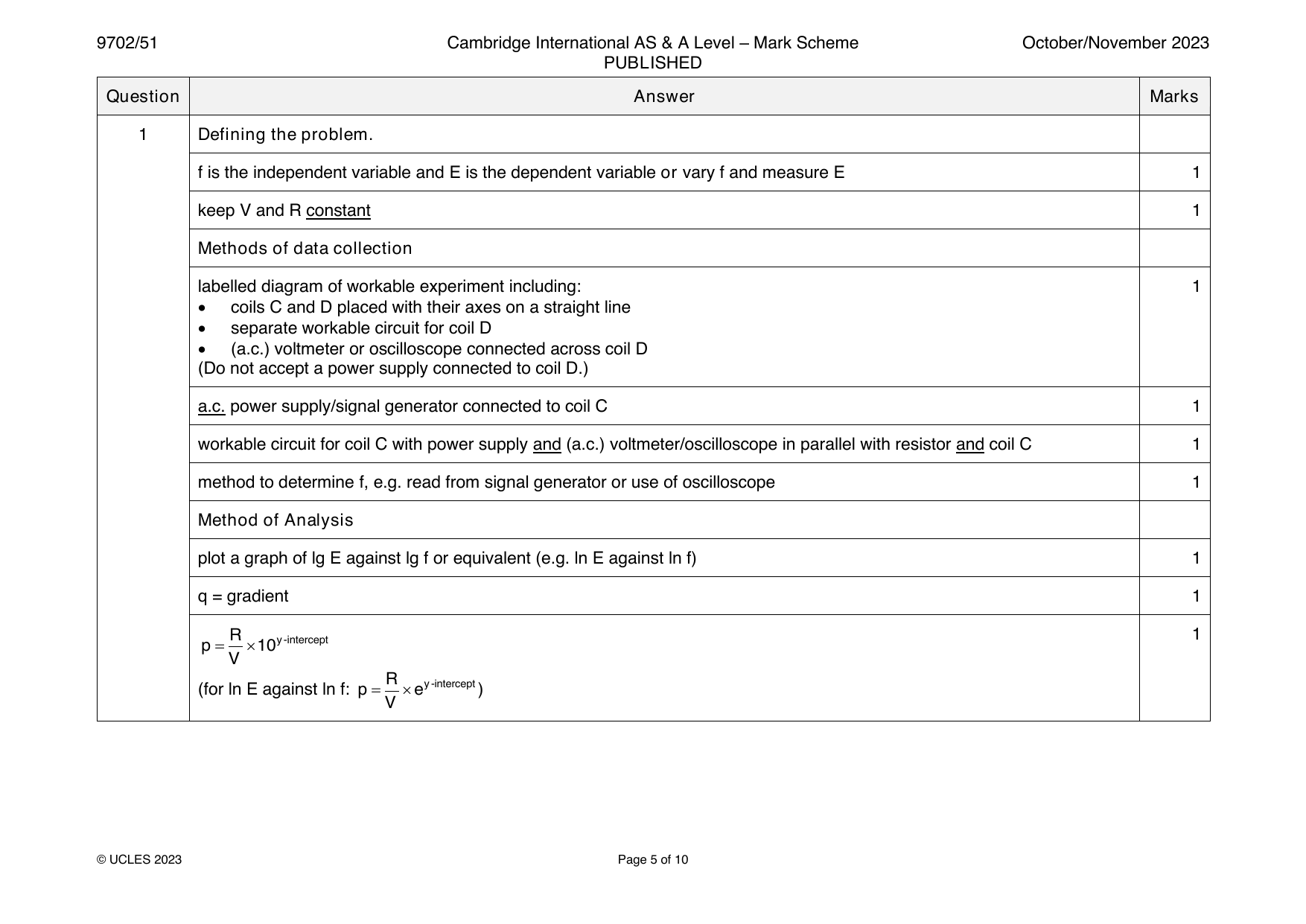
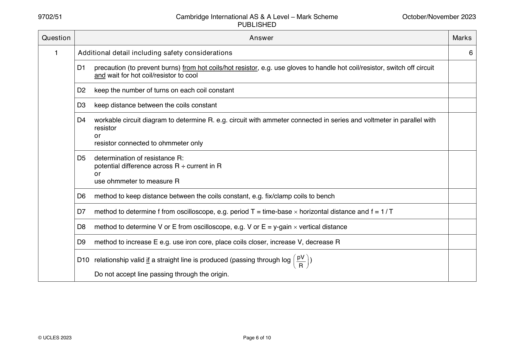
1 Defining the problem.
f is the independent variable and E is the dependent variable or vary f and measure E 1
keep V and R constant 1
Methods of data collection
labelled diagram of workable experiment including: 1
• coils C and D placed with their axes on a straight line
• separate workable circuit for coil D
• (a.c.) voltmeter or oscilloscope connected across coil D
(Do not accept a power supply connected to coil D.)
a.c. power supply/signal generator connected to coil C 1
workable circuit for coil C with power supply and (a.c.) voltmeter/oscilloscope in parallel with resistor and coil C 1
method to determine f, e.g. read from signal generator or use of oscilloscope 1
Method of Analysis
plot a graph of lg E against lg f or equivalent (e.g. ln E against ln f) 1
q = gradient 1
R 1
p= 10y-intercept
V
R
(for ln E against ln f: p= ey-intercept)
V
© UCLES 2023 Page 5 of 10
1 Additional detail including safety considerations 6
D1 precaution (to prevent burns) from hot coils/hot resistor, e.g. use gloves to handle hot coil/resistor, switch off circuit
and wait for hot coil/resistor to cool
D2 keep the number of turns on each coil constant
D3 keep distance between the coils constant
D4 workable circuit diagram to determine R. e.g. circuit with ammeter connected in series and voltmeter in parallel with
resistor
or
resistor connected to ohmmeter only
D5 determination of resistance R:
potential difference across R ÷ current in R
or
use ohmmeter to measure R
D6 method to keep distance between the coils constant, e.g. fix/clamp coils to bench
D7 method to determine f from oscilloscope, e.g. period T = time-base horizontal distance and f = 1 / T
D8 method to determine V or E from oscilloscope, e.g. V or E = y-gain vertical distance
D9 method to increase E e.g. use iron core, place coils closer, increase V, decrease R
pV
D10 relationship valid if a straight line is produced (passing through log )
R
Do not accept line passing through the origin.
© UCLES 2023 Page 6 of 10
Official mark scheme pages: 5, 6 · source PDF URL
9702-2023-on-51-q02
Oct/Nov 2023 · Paper 51 · Question 2 · 15 marks
2(a) 2g 1
gradient =
uZ
2g
y-intercept =
u
2(b) 1
1
1 −
/cm 2
h
0.218 or 0.2182
0.237 or 0.2370
0.248 or 0.2485
0.262 or 0.2617
0.282 or 0.2817
0.313 or 0.3131
Values correct as shown above.
1 1
Uncertainties in from ± 0.001 to ± 0.003.
h
2(c)(i) Six points from (b) plotted correctly. 1
Must be within half a small square. Diameter of points must be less than half a small square.
1 1
Error bars in plotted correctly.
h
All error bars to be plotted. Total length of bar must be accurate to less than half a small square and symmetrical.
© UCLES 2023 Page 7 of 10
2(c)(ii) Straight line of best fit drawn. 1
Do not accept line from top point to bottom point.
Points must be balanced.
Line must pass between (605, 0.230) and (615, 0.230) and between (845, 0.300) and (855, 0.300)
Worst acceptable line drawn (steepest or shallowest possible line that passes through all the error bars). 1
All error bars must be plotted.
2(c)(iii) Gradient determined with clear substitution of data points into y / x. 1
Distance between data points must be greater than half the length of the drawn line.
Gradient determined of worst acceptable line. 1
uncertainty = (gradient of line of best fit – gradient of worst acceptable line)
or
uncertainty = ½ (steepest worst line gradient – shallowest worst line gradient)
2(c)(iv) y-intercept determined by substitution of correct point with consistent power of ten into y = mx + c. 1
y-intercept of worst acceptable line determined by substitution into y = mx + c. 1
uncertainty = y-intercept of line of best fit – y-intercept of worst acceptable line
or
uncertainty = ½ (steepest worst line y-intercept – shallowest worst line y-intercept)
Do not accept ECF from false origin method.
© UCLES 2023 Page 8 of 10
2(d)(i) u determined using y-intercept and u and Z given to 2, 3 or 4 significant figures. 1
2981 44.29
u = =
y-intercept (c)(iv)
Z determined using gradient with method shown and u and Z given with SI units with appropriate powers of ten. 1
2981 44.29 y-intercept (c)(iv)
Z = = or Z = =
u gradient u(c)(iii) gradient (c)(iii)
2(d)(ii) Percentage uncertainty in Z with method shown. 1
y-intercept gradient
percentage uncertainty in Z = + 100
y-intercept gradient
or
Correct substitution for u and
u gradient
percentage uncertainty in Z = + 100
u gradient
or
Correct substitution for max/min methods.
© UCLES 2023 Page 9 of 10
2(e) M determined to a minimum of 2 significant figures from (c)(iii) and (c)(iv) or (d)(i) with correct substitution. 1
1
−y-intercept
25
M =
gradient
or
uZ uZ
M = −Z = −Z
2gh 221.5
© UCLES 2023 Page 10 of 10
Official mark scheme pages: 7, 8, 9, 10 · source PDF URL
9702-2023-on-52-q01
Oct/Nov 2023 · Paper 52 · Question 1 · 15 marks
1 Defining the problem
V is the independent variable and z is the dependent variable or vary V and measure z 1
keep h constant 1
Methods of data collection
labelled diagram of workable experiment including: 1
• pulley supported by stand
• stand placed on surface/bench/floor
• minimum of two labels from stand, beaker, oil, surface/bench/floor, pulley, string
use (metre) rule to measure h or (metre) rule correctly positioned with h marked on diagram 1
use measuring cylinder to measure V 1
timing method to measure time t of fall of beaker to determine z 1
e.g. use timer/stopwatch or use light gate(s) connected to a timer/data logger
© UCLES 2023 Page 5 of 11
1 Method of Analysis
1 1 1 1 1
plot a graph of against or equivalent (e.g. against )
z2 V V z2
Do not accept logarithms.
1 1
b=
2hy-intercept
1 1 Mgradient gradient
(for against :b= or b=− )
V z2 ah 2hy-intercept
M 2My-intercept 1
a= or a=
bhgradient gradient
1 1
(for against : a=−2My-intercept)
V z2
© UCLES 2023 Page 6 of 11
1 Additional detail including safety considerations 6
D1 precaution linked to oil spillage, e.g. use of cushion/sand box/tray for falling beaker to land or use of bungs/lids on
beakers or use foam on bench/floor or use foam to prevent rising beaker hitting pulley
D2 precaution linked to oil contact with skin e.g. use gloves to avoid contact with oil
D3 keep M constant
D4 use a (top-pan) balance to measure M
D5 method to keep h constant e.g. use a fiducial mark to release the beaker from the same position or release from the
same position on the clamped rule each time
D6 equation to determine z for method used, e.g.
for timing h, z = 2h / t
or
for one light gate, z = L / t where L is the length of the interrupted beam
or
for two light gates, z = distance between light gates / t
Do not accept h / t.
D7 additional detail on diagram to measure h, e.g. clamp (metre) rule with stand on surface or use of set squares
positioned on the surface to side of rule or spirit level positioned to side of rule
D8 use large value of h to increase time of fall of beaker
D9 repeat measurements of z for the same V and average z
1
D10 relationship valid if a straight line is produced (passing through )
2bh
Do not accept line passing through the origin.
© UCLES 2023 Page 7 of 11
Official mark scheme pages: 5, 6, 7 · source PDF URL
9702-2023-on-52-q02
Oct/Nov 2023 · Paper 52 · Question 2 · 15 marks
2(a) t 1
gradient = −
R
y-intercept = ln I R
0
2(b) 1
1 / C / 104 F–1 ln (V / V)
0.91 or 0.909 0.896 or 0.8961
0.76 or 0.758 1.012 or 1.0116
0.63 or 0.633 1.115 or 1.1151
0.61 or 0.606 1.131 or 1.1314
0.48 or 0.482 1.253 or 1.2528
0.36 or 0.357 1.348 or 1.3481
Values correct as shown above.
Uncertainties in ln (V / V) from ± 0.021 or ± 0.020 to ± 0.010 or ± 0.013 1
2(c)(i) Six points from (b) plotted correctly. 1
Must be within half a small square. Diameter of points must be less than half a small square.
Error bars in ln (V / V) plotted correctly. 1
All error bars to be plotted. Total length of bar must be accurate to less than half a small square and symmetrical.
© UCLES 2023 Page 8 of 11
2(c)(ii) Straight line of best fit drawn. 1
Do not accept line from top point to bottom point.
Points must be balanced.
Line must pass between (0.820, 0.95) and (0.845, 0.95) and between (0.400, 1.30) and (0.425, 1.30)
Worst acceptable line drawn (steepest or shallowest possible line that passes through all the error bars). 1
All error bars must be plotted.
2(c)(iii) Gradient determined with clear substitution of data points into y / x. 1
Distance between data points must be greater than half the length of the drawn line.
Gradient must be negative.
Gradient determined of worst acceptable line. 1
uncertainty = (gradient of line of best fit – gradient of worst acceptable line)
or
uncertainty = ½ (steepest worst line gradient – shallowest worst line gradient)
2(c)(iv) y-intercept determined by substitution of correct point with consistent power of ten in m and x into y = mx + c. 1
© UCLES 2023 Page 9 of 11
2(d)(i) R determined using gradient. 1
30.0 30.0
R =− =
gradient (c)(iii)
I determined using y-intercept with method shown. 1
0
ey-intercept e(c)(iv)
I = =
0 R (d)(i)
R and I determined correctly using gradient and y-intercept 1
0
and
R and I given to 2 or 3 significant figures
0
and
R and I given with SI units with appropriate powers of ten.
0
Units:
R: or s F-1
I : A or V F s–1 or V –1
0
2(d)(ii) Percentage uncertainty in R with method shown. 1
t gradient
percentage uncertainty in R= + 100
t gradient
or
Correct substitution for max/min methods.
© UCLES 2023 Page 10 of 11
2(e) C determined to a minimum of 2 significant figures from (c)(iii) and (c)(iv) or (d)(i) with correct substitutions. 1
gradient gradient
C = or C =−
lnV −y-intercept y-intercept−lnV
or
t t
C =− or C =
R(lnV −lnI R) R(lnI R −lnV)
0 0
© UCLES 2023 Page 11 of 11
Official mark scheme pages: 8, 9, 10, 11 · source PDF URL
9702-2023-on-53-q01
Oct/Nov 2023 · Paper 53 · Question 1 · 15 marks
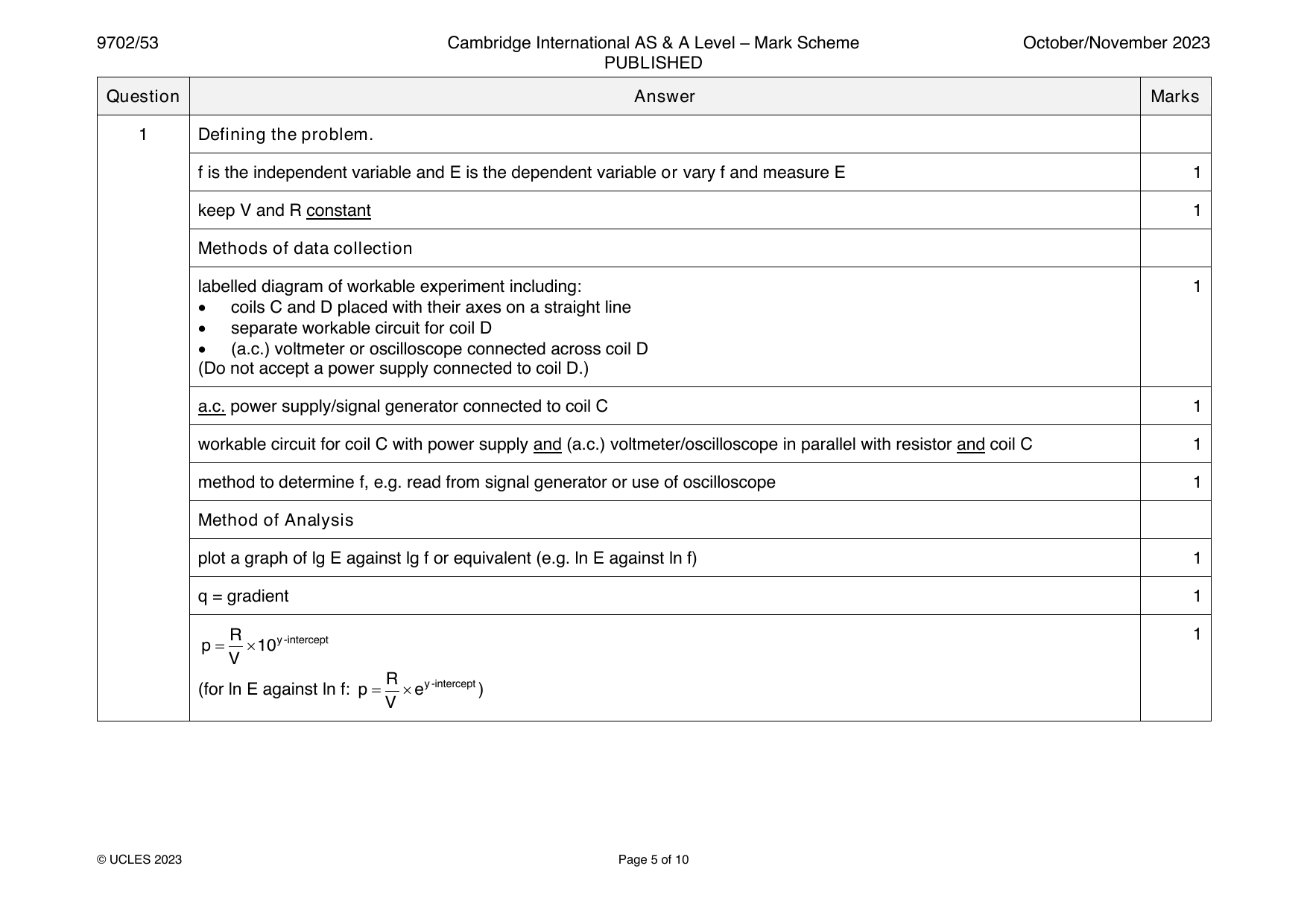
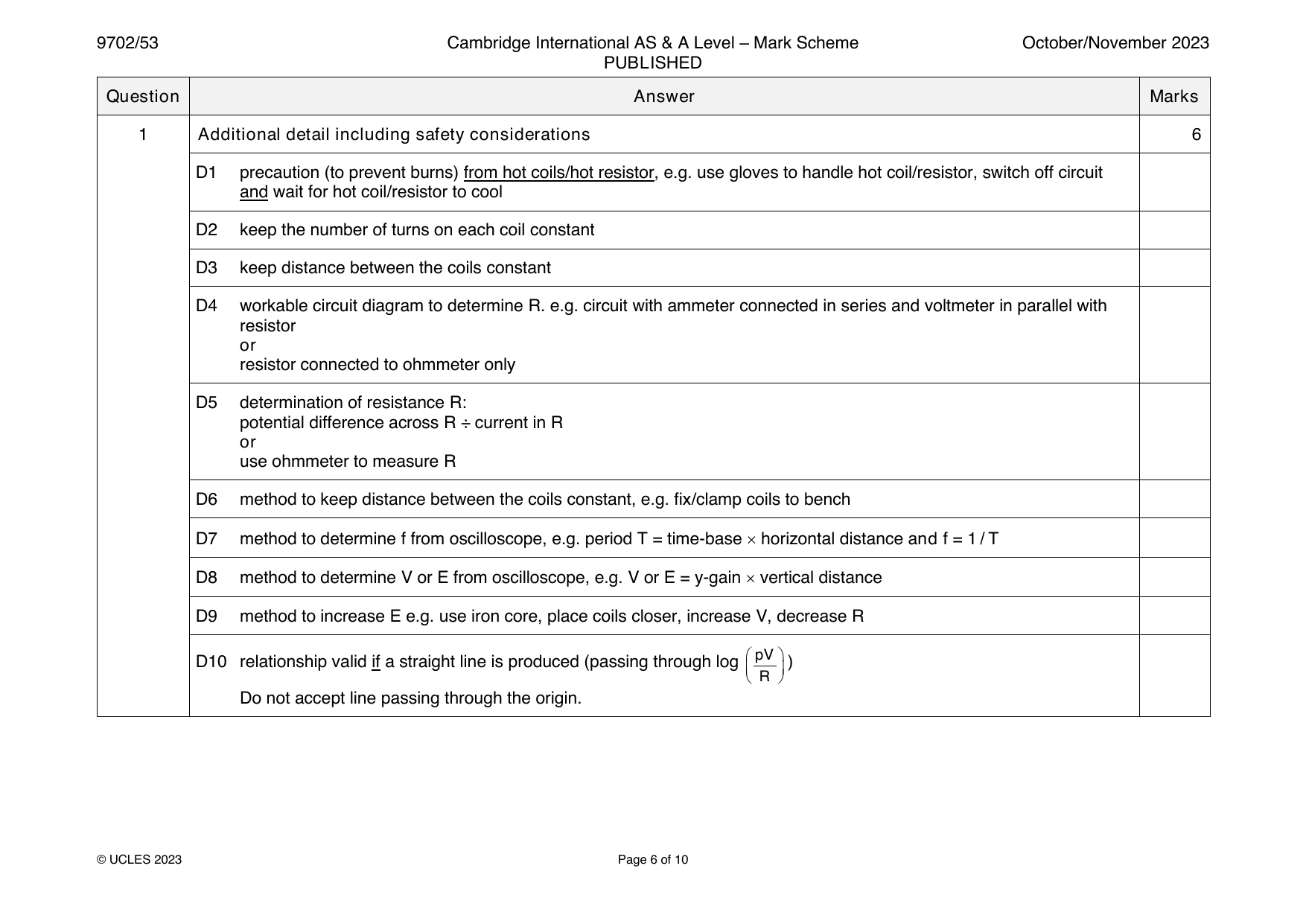
1 Defining the problem.
f is the independent variable and E is the dependent variable or vary f and measure E 1
keep V and R constant 1
Methods of data collection
labelled diagram of workable experiment including: 1
• coils C and D placed with their axes on a straight line
• separate workable circuit for coil D
• (a.c.) voltmeter or oscilloscope connected across coil D
(Do not accept a power supply connected to coil D.)
a.c. power supply/signal generator connected to coil C 1
workable circuit for coil C with power supply and (a.c.) voltmeter/oscilloscope in parallel with resistor and coil C 1
method to determine f, e.g. read from signal generator or use of oscilloscope 1
Method of Analysis
plot a graph of lg E against lg f or equivalent (e.g. ln E against ln f) 1
q = gradient 1
R 1
p= 10y-intercept
V
R
(for ln E against ln f: p= ey-intercept)
V
© UCLES 2023 Page 5 of 10
1 Additional detail including safety considerations 6
D1 precaution (to prevent burns) from hot coils/hot resistor, e.g. use gloves to handle hot coil/resistor, switch off circuit
and wait for hot coil/resistor to cool
D2 keep the number of turns on each coil constant
D3 keep distance between the coils constant
D4 workable circuit diagram to determine R. e.g. circuit with ammeter connected in series and voltmeter in parallel with
resistor
or
resistor connected to ohmmeter only
D5 determination of resistance R:
potential difference across R ÷ current in R
or
use ohmmeter to measure R
D6 method to keep distance between the coils constant, e.g. fix/clamp coils to bench
D7 method to determine f from oscilloscope, e.g. period T = time-base horizontal distance and f = 1 / T
D8 method to determine V or E from oscilloscope, e.g. V or E = y-gain vertical distance
D9 method to increase E e.g. use iron core, place coils closer, increase V, decrease R
pV
D10 relationship valid if a straight line is produced (passing through log )
R
Do not accept line passing through the origin.
© UCLES 2023 Page 6 of 10
Official mark scheme pages: 5, 6 · source PDF URL
9702-2023-on-53-q02
Oct/Nov 2023 · Paper 53 · Question 2 · 15 marks
2(a) 2g 1
gradient =
uZ
2g
y-intercept =
u
2(b) 1
1
1 −
/cm 2
h
0.218 or 0.2182
0.237 or 0.2370
0.248 or 0.2485
0.262 or 0.2617
0.282 or 0.2817
0.313 or 0.3131
Values correct as shown above.
1 1
Uncertainties in from ± 0.001 to ± 0.003.
h
2(c)(i) Six points from (b) plotted correctly. 1
Must be within half a small square. Diameter of points must be less than half a small square.
1 1
Error bars in plotted correctly.
h
All error bars to be plotted. Total length of bar must be accurate to less than half a small square and symmetrical.
© UCLES 2023 Page 7 of 10
2(c)(ii) Straight line of best fit drawn. 1
Do not accept line from top point to bottom point.
Points must be balanced.
Line must pass between (605, 0.230) and (615, 0.230) and between (845, 0.300) and (855, 0.300)
Worst acceptable line drawn (steepest or shallowest possible line that passes through all the error bars). 1
All error bars must be plotted.
2(c)(iii) Gradient determined with clear substitution of data points into y / x. 1
Distance between data points must be greater than half the length of the drawn line.
Gradient determined of worst acceptable line. 1
uncertainty = (gradient of line of best fit – gradient of worst acceptable line)
or
uncertainty = ½ (steepest worst line gradient – shallowest worst line gradient)
2(c)(iv) y-intercept determined by substitution of correct point with consistent power of ten into y = mx + c. 1
y-intercept of worst acceptable line determined by substitution into y = mx + c. 1
uncertainty = y-intercept of line of best fit – y-intercept of worst acceptable line
or
uncertainty = ½ (steepest worst line y-intercept – shallowest worst line y-intercept)
Do not accept ECF from false origin method.
© UCLES 2023 Page 8 of 10
2(d)(i) u determined using y-intercept and u and Z given to 2, 3 or 4 significant figures. 1
2981 44.29
u = =
y-intercept (c)(iv)
Z determined using gradient with method shown and u and Z given with SI units with appropriate powers of ten. 1
2981 44.29 y-intercept (c)(iv)
Z = = or Z = =
u gradient u(c)(iii) gradient (c)(iii)
2(d)(ii) Percentage uncertainty in Z with method shown. 1
y-intercept gradient
percentage uncertainty in Z = + 100
y-intercept gradient
or
Correct substitution for u and
u gradient
percentage uncertainty in Z = + 100
u gradient
or
Correct substitution for max/min methods.
© UCLES 2023 Page 9 of 10
2(e) M determined to a minimum of 2 significant figures from (c)(iii) and (c)(iv) or (d)(i) with correct substitution. 1
1
−y-intercept
25
M =
gradient
or
uZ uZ
M = −Z = −Z
2gh 221.5
© UCLES 2023 Page 10 of 10
Official mark scheme pages: 7, 8, 9, 10 · source PDF URL
9702-2024-m-52-q01
March 2024 · Paper 52 · Question 1 · 15 marks
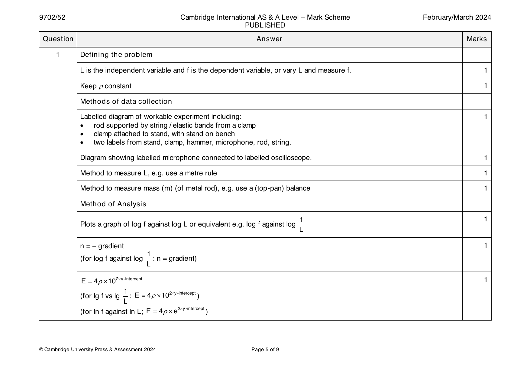
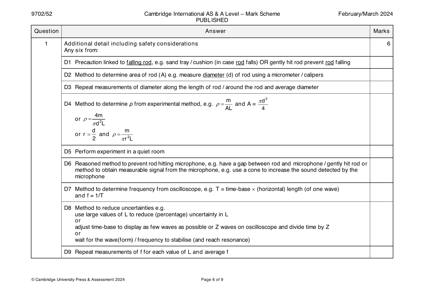
1 Defining the problem
L is the independent variable and f is the dependent variable, or vary L and measure f. 1
Keep constant 1
Methods of data collection
Labelled diagram of workable experiment including: 1
• rod supported by string / elastic bands from a clamp
• clamp attached to stand, with stand on bench
• two labels from stand, clamp, hammer, microphone, rod, string.
Diagram showing labelled microphone connected to labelled oscilloscope. 1
Method to measure L, e.g. use a metre rule 1
Method to measure mass (m) (of metal rod), e.g. use a (top-pan) balance 1
Method of Analysis
1 1
Plots a graph of log f against log L or equivalent e.g. log f against log
L
n = − gradient 1
1
(for log f against log : n = gradient)
L
E =4102y-intercept 1
1
(for lg f vs lg : E =4102y-intercept)
L
(for ln f against ln L; E =4e2y-intercept)
© Cambridge University Press & Assessment 2024 Page 5 of 9
1 Additional detail including safety considerations 6
Any six from:
D1 Precaution linked to falling rod, e.g. sand tray / cushion (in case rod falls) OR gently hit rod prevent rod falling
D2 Method to determine area of rod (A) e.g. measure diameter (d) of rod using a micrometer / calipers
D3 Repeat measurements of diameter along the length of rod / around the rod and average diameter
m d2
D4 Method to determine ρ from experimental method, e.g. = and A =
AL 4
4m
or =
d2L
d m
or r = and =
Official mark scheme pages: 5, 6 · source PDF URL
9702-2024-m-52-q02
March 2024 · Paper 52 · Question 2 · 15 marks
2 r2L
D5 Perform experiment in a quiet room
D6 Reasoned method to prevent rod hitting microphone, e.g. have a gap between rod and microphone / gently hit rod or
method to obtain measurable signal from the microphone, e.g. use a cone to increase the sound detected by the
microphone
D7 Method to determine frequency from oscilloscope, e.g. T = time-base (horizontal) length (of one wave)
and f = 1/T
D8 Method to reduce uncertainties e.g.
use large values of L to reduce (percentage) uncertainty in L
or
adjust time-base to display as few waves as possible or Z waves on oscilloscope and divide time by Z
or
wait for the wave(form) / frequency to stabilise (and reach resonance)
D9 Repeat measurements of f for each value of L and average f
© Cambridge University Press & Assessment 2024 Page 6 of 9
2(a) 3 1
Gradient =
E
4Z
y-intercept =
E
2(b) 1
1
/ A−1
I
4440 or 4444
5410 or 5405
6250 or 6250
7140 or 7143
8000 or 8000
8700 or 8696
1 1
Uncertainties in
I
From 90–110 to 360–400
© Cambridge University Press & Assessment 2024 Page 7 of 9
2(c)(i) Six points from (b) plotted correctly. 1
Must be within half a small square. Diameter of points must be less than half a small square.
1 1
Error bars in plotted correctly.
I
All error bars to be plotted. Total length of bar must be accurate to less than half a small square and symmetrical.
2(c)(ii) Straight line of best fit drawn. 1
Do not accept line from top plot to bottom plot.
Points must be balanced.
Line must pass between (1.8, 5000) and (2.1, 5000) and between (7.2, 8500) and (7.5, 8500)
Worst acceptable line drawn. 1
Steepest or shallowest possible line that passes through all the error bars.
All error bars must be plotted.
2(c)(iii) Gradient determined with clear substitution of data points into y / x; distance between data points must be greater than 1
half the length of the drawn line.
Gradient determined of worst acceptable line with clear substitution of data points into y / x; 1
uncertainty = (gradient of line of best fit – gradient of worst acceptable line)
or
uncertainty = ½ (steepest worst line gradient – shallowest worst line gradient)
2(c)(iv) y-intercept determined by substitution of correct point with consistent power of ten in m and x into y = mx + c 1
y-intercept of worst acceptable line determined by substitution into y = mx + c 1
uncertainty = y-intercept of line of best fit – y-intercept of worst acceptable line, or
uncertainty = ½ (steepest worst line y-intercept – shallowest worst line y-intercept)
© Cambridge University Press & Assessment 2024 Page 8 of 9
2(d)(i) E determined using gradient and 1
E and Z given to 2, 3 or 4 sf.
3
E =
gradient
Z determined using y-intercept and 1
E and Z given with SI units with correct powers of ten
Ey-intercept 3 y-intercept
Z = or Z =
4 4 gradient
Unit of E: V or A
Unit of Z:
2(d)(ii) Percentage uncertainty in Z with method shown. 1
gradient y-intercept
%uncertainty= +
gradient y-intercept
or
Correct substitution for max/min methods.
2(e) R determined to a minimum of 2sf from (c)(iii) and (c)(iv) or (d)(i) with correct substitution and correct powers of ten. 1
0.1 mA = 0.1 10–3 A and
1
− y-intercept
0.1010−3
R = or
gradient
E 4Z
R = −
30.1010−3 3
© Cambridge University Press & Assessment 2024 Page 9 of 9
Official mark scheme pages: 6, 7, 8, 9 · source PDF URL
9702-2024-mj-51-q01
May/June 2024 · Paper 51 · Question 1 · 15 marks
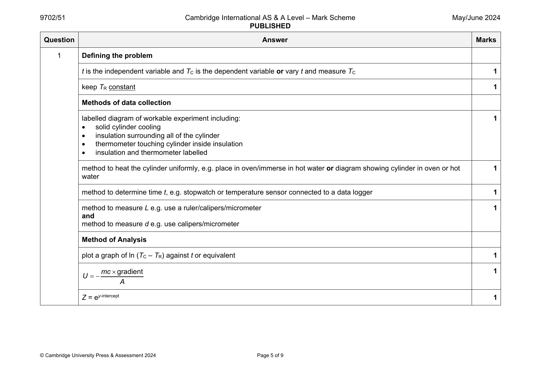
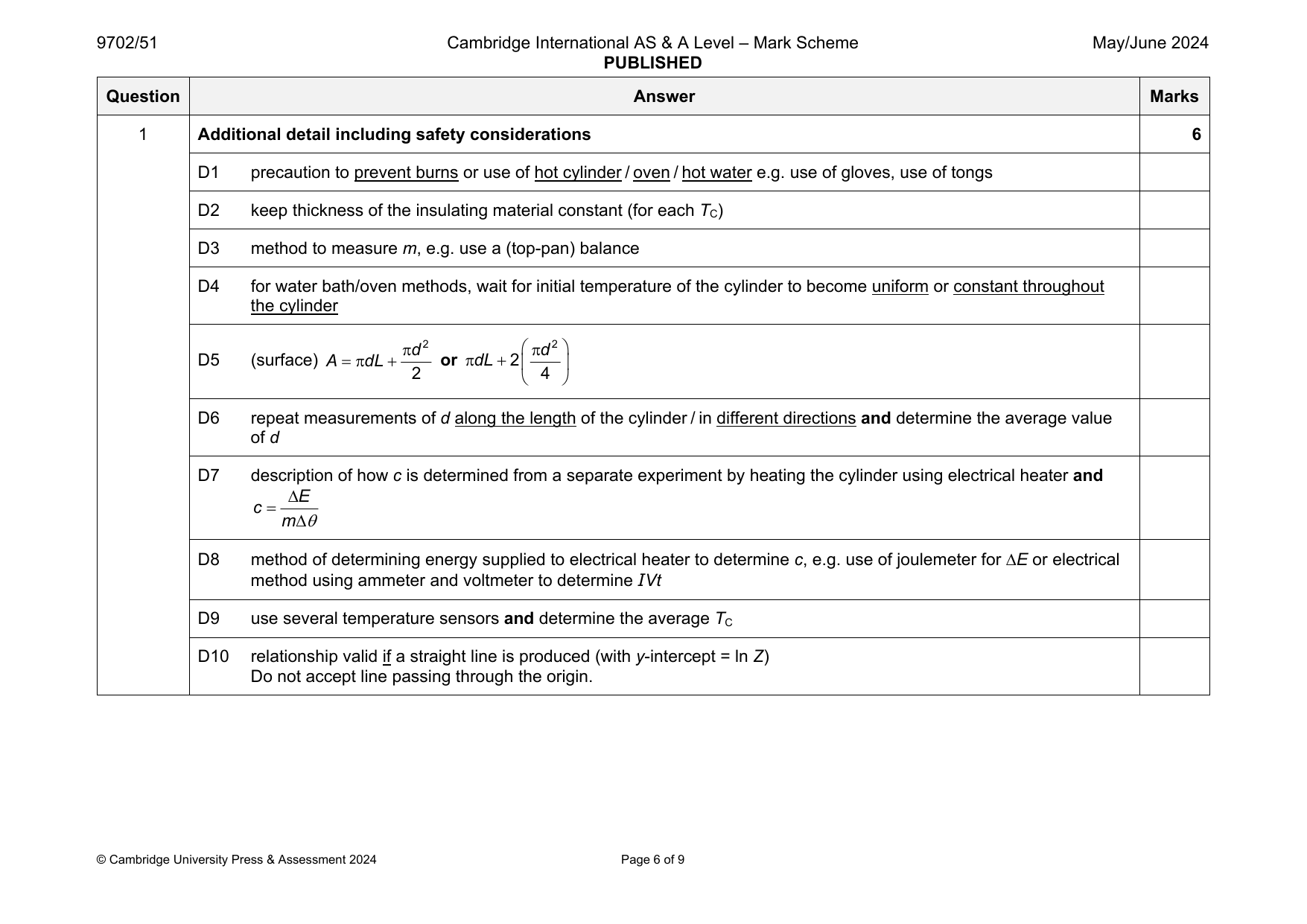
1 Defining the problem
t is the independent variable and T is the dependent variable or vary t and measure T 1
C C
keep T constant 1
R
Methods of data collection
labelled diagram of workable experiment including: 1
solid cylinder cooling
insulation surrounding all of the cylinder
thermometer touching cylinder inside insulation
insulation and thermometer labelled
method to heat the cylinder uniformly, e.g. place in oven/immerse in hot water or diagram showing cylinder in oven or hot 1
water
method to determine time t, e.g. stopwatch or temperature sensor connected to a data logger 1
method to measure L e.g. use a ruler/calipers/micrometer 1
and
method to measure d e.g. use calipers/micrometer
Method of Analysis
plot a graph of ln (T – T ) against t or equivalent 1
C R
mcgradient 1
U
A
Z = ey-intercept 1
© Cambridge University Press & Assessment 2024 Page 5 of 9
1 Additional detail including safety considerations 6
D1 precaution to prevent burns or use of hot cylinder / oven / hot water e.g. use of gloves, use of tongs
D2 keep thickness of the insulating material constant (for each T )
C
D3 method to measure m, e.g. use a (top-pan) balance
D4 for water bath/oven methods, wait for initial temperature of the cylinder to become uniform or constant throughout
the cylinder
d2 d2
D5 (surface) AdL or dL2
Official mark scheme pages: 5, 6 · source PDF URL
9702-2024-mj-51-q02
May/June 2024 · Paper 51 · Question 2 · 15 marks
2 4
D6 repeat measurements of d along the length of the cylinder / in different directions and determine the average value
of d
D7 description of how c is determined from a separate experiment by heating the cylinder using electrical heater and
E
c
m
D8 method of determining energy supplied to electrical heater to determine c, e.g. use of joulemeter for E or electrical
method using ammeter and voltmeter to determine IVt
D9 use several temperature sensors and determine the average T
C
D10 relationship valid if a straight line is produced (with y-intercept = ln Z)
Do not accept line passing through the origin.
© Cambridge University Press & Assessment 2024 Page 6 of 9
2(a) 1 1
gradient =
kf
s
1
y-intercept =
f
s
2(b) 1
1
v / ms–1 / 10–3 Hz–1
f
3.5 0.4 1.118 or 1.1183
6.3 0.4 1.110 or 1.1096
8.7 0.5 1.101 or 1.1013
11.4 0.5 1.092 or 1.0919
13.9 0.6 1.083 or 1.0827
16.2 0.6 1.074 or 1.0739
1
Values of v and correct as shown above.
f
Uncertainties in v correct as shown above. 1
2(c)(i) Six points from (b) plotted correctly. 1
Must be within half a small square. Diameter of points must be less than half a small square.
Error bars in v plotted correctly. 1
All error bars to be plotted. Total length of bar must be accurate to less than half a small square and symmetrical.
© Cambridge University Press & Assessment 2024 Page 7 of 9
2(c)(ii) Straight line of best fit drawn. 1
Do not accept line from top point to bottom point.
Line must pass between (14.5, 1.080) and (14.9, 1.080) and between (4.5, 1.115) and (4.8, 1.115).
Worst acceptable line drawn (steepest or shallowest possible line that passes through all the error bars). 1
All error bars must be plotted.
2(c)(iii) Gradient determined with clear substitution of data points into y / x. 1
Gradient must be negative.
Distance between data points must be greater than half the length of the drawn line.
Gradient determined of worst acceptable line with clear substitution of data points into y / x. 1
uncertainty = (gradient of line of best fit – gradient of worst acceptable line)
or
uncertainty = ½ (steepest worst line gradient – shallowest worst line gradient)
2(c)(iv) y-intercept determined by substitution of correct point with consistent power of ten in m and y into y = mx + c. 1
y-intercept of worst acceptable line determined by substitution into y = mx + c. 1
uncertainty = y-intercept of line of best fit – y-intercept of worst acceptable line
or
uncertainty = ½ (steepest worst line y-intercept – shallowest worst line y-intercept)
Do not accept ECF from false origin method.
© Cambridge University Press & Assessment 2024 Page 8 of 9
2(d)(i) f determined using y-intercept and f given to 2, 3 or 4 significant figures and k given to 2 or 3 significant figures. 1
s s
1
f
s y-intercept
k determined using gradient with method shown and f and k given with SI units with appropriate powers of ten. 1
s
y-intercept 1
k or k
gradient gradientf
s
Units of f : Hz
s
Units of k: m s–1
2(d)(ii) Percentage uncertainty in k with method shown. 1
y-intercept gradient
percentage uncertainty 100
y-intercept gradient
or
correct substitution for max/min methods.
2(e) v determined (non-zero) to a minimum of 2 significant figures from (c)(iii) and (c)(iv) or (d)(i) with correct substitution. 1
1
y-intercept
f
v
gradient
or
kf
v k s
f
© Cambridge University Press & Assessment 2024 Page 9 of 9
Official mark scheme pages: 6, 7, 8, 9 · source PDF URL
9702-2024-mj-52-q01
May/June 2024 · Paper 52 · Question 1 · 15 marks
1 Defining the problem
t is the independent variable and s is the dependent variable or vary t and measure s 1
keep k constant 1
Methods of data collection
labelled diagram of workable experiment including: 1
spring connected to magnet
vertical rule parallel to spring to determine s
rule held in position by a stand
stand resting on the bench
rule labelled and at least one other label from stand, clamp, card, (magnetic) sheet, (cylindrical) magnet, spring
s = (new) length/position of spring – original length/position of spring 1
use a micrometer to measure t 1
measure B using a (calibrated) Hall probe and rotate probe until maximum value 1
or
measure B using Hall probe first in one direction, then in the opposite direction and average
© Cambridge University Press & Assessment 2024 Page 5 of 10
1 Method of Analysis
1 1
plot a graph of s against or equivalent
t
(allow lg s against lg t)
relationship valid if a straight line that passes through the origin is produced 1
(for lg s against lg t: relationship valid if a straight line with gradient 1)
k 1
Z gradient
ALB
k10y-intercept
(for lg s against lg t: Z )
ALB
© Cambridge University Press & Assessment 2024 Page 6 of 10
1 Additional detail including safety considerations 6
D1 precaution related to spring and/or magnet hitting eyes, e.g. use of goggles/use of safety screen around experiment
D2 keep A, L and B constant
D3 use a rule to measure L
D4 micrometer/calipers to measure diameter d of the magnet and A = d2 / 4
D5 description of method to determine k, e.g. add mass to spring and k = mg / extension
or
use newton meter to measure force applied to spring and k = force / extension
or
take several readings of force and extension, plot a force–extension graph and k = gradient
D6 (magnetic) sheet clamped to bench
D7 use pointer(s)/marker(s) on the spring to read off values from the rule
D8 method to use video recorder and replay to determine maximum length of the spring
or
increase s or force gradually/slowly until magnet (just) leaves the card
D9 repeat measurements of t in different positions on the card and average t
or
repeat measurements of s for each value of t and average s
D10 method to check that the spring has not exceeded the elastic limit
D11 use of non-magnetic stand or named non-magnetic material for stand, e.g. wood
© Cambridge University Press & Assessment 2024 Page 7 of 10
Official mark scheme pages: 5, 6, 7 · source PDF URL
9702-2024-mj-52-q02
May/June 2024 · Paper 52 · Question 2 · 15 marks
2(a) gradient = n 1
2
y-intercept = lg
C
2(b) 1
lg (L / cm) lg (T / 10–5 s)
1.73 or 1.732 1.38 or 1.380 0.02
1.85 or 1.845 1.51 or 1.505 0.01
1.93 or 1.934 1.59 or 1.591 0.01
2.033 or 2.0334 1.69 or 1.690 0.02
2.146 or 2.1461 1.81 or 1.806 0.01
2.223 or 2.2227 1.87 or 1.869 0.01
Values of lg (L/ cm) and lg (T/ 10–5 s) correct as shown above.
Uncertainties in lg (T/ 10–5 s) correct as shown above. 1
2(c)(i) Six points from (b) plotted correctly. 1
Must be within half a small square. Diameter of points must be less than half a small square.
Error bars in lg T plotted correctly. 1
All error bars to be plotted. Total length of bar must be accurate to less than half a small square and symmetrical.
© Cambridge University Press & Assessment 2024 Page 8 of 10
2(c)(ii) Straight line of best fit drawn. 1
Do not accept line from top point to bottom point.
Line must pass between (1.780, 1.45) and (1.800, 1.45) and between (2.085, 1.75) and (2.100, 1.75)
Worst acceptable line drawn (steepest or shallowest possible line that passes through all the error bars). 1
All error bars must be plotted.
2(c)(iii) Gradient determined with clear substitution of data points into y / x. 1
Distance between data points must be greater than half the length of the drawn line.
Gradient determined of worst acceptable line with clear substitution of data points into y / x. 1
uncertainty = (gradient of line of best fit – gradient of worst acceptable line)
or
uncertainty = ½ (steepest worst line gradient – shallowest worst line gradient)
2(c)(iv) y-intercept determined by substitution of correct point with consistent power of ten in m and x into y = mx + c. 1
y-intercept of worst acceptable line determined by substitution into y = mx + c. 1
uncertainty = y-intercept of line of best fit – y-intercept of worst acceptable line
or
uncertainty = ½ (steepest worst line y-intercept – shallowest worst line y-intercept)
Do not accept ECF from false origin method.
© Cambridge University Press & Assessment 2024 Page 9 of 10
2(d) Value of n determined using gradient (n = gradient) and C given to 2 or 3 significant figures. 1
Value of C determined using y-intercept with method shown. 1
2
C
10y-intercept
Absolute uncertainties in n and C. 1
uncertainty in n = uncertainty in gradient
and
2 2
2 10minworst y-intercept 10maxworst y-intercept
C=C or C =
10worst y-intercept 2
Clear method must be shown with C correctly evaluated.
2(e) Value of L determined (non-zero) to a minimum of 2 significant figures from (c)(iii) and (c)(iv) or (d) with correct substitution 1
and correct power of ten.
Units of T and either C or y-intercept must be consistent.
2
logT log
C log10y-intercept
logL
n n
log10y-intercept
L10 n
or
TC
L n
2
© Cambridge University Press & Assessment 2024 Page 10 of 10
Official mark scheme pages: 8, 9, 10 · source PDF URL
9702-2024-mj-53-q01
May/June 2024 · Paper 53 · Question 1 · 15 marks
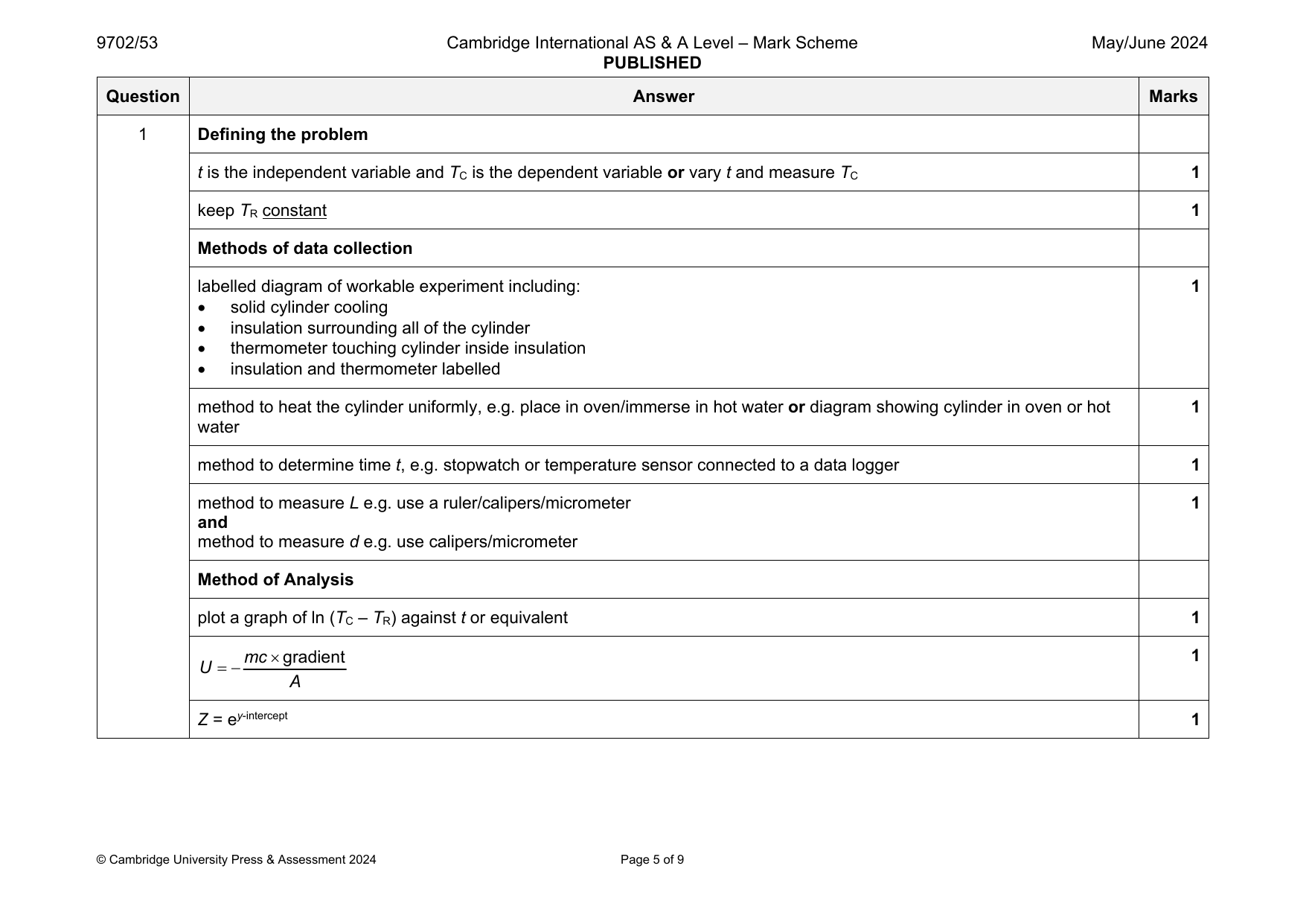
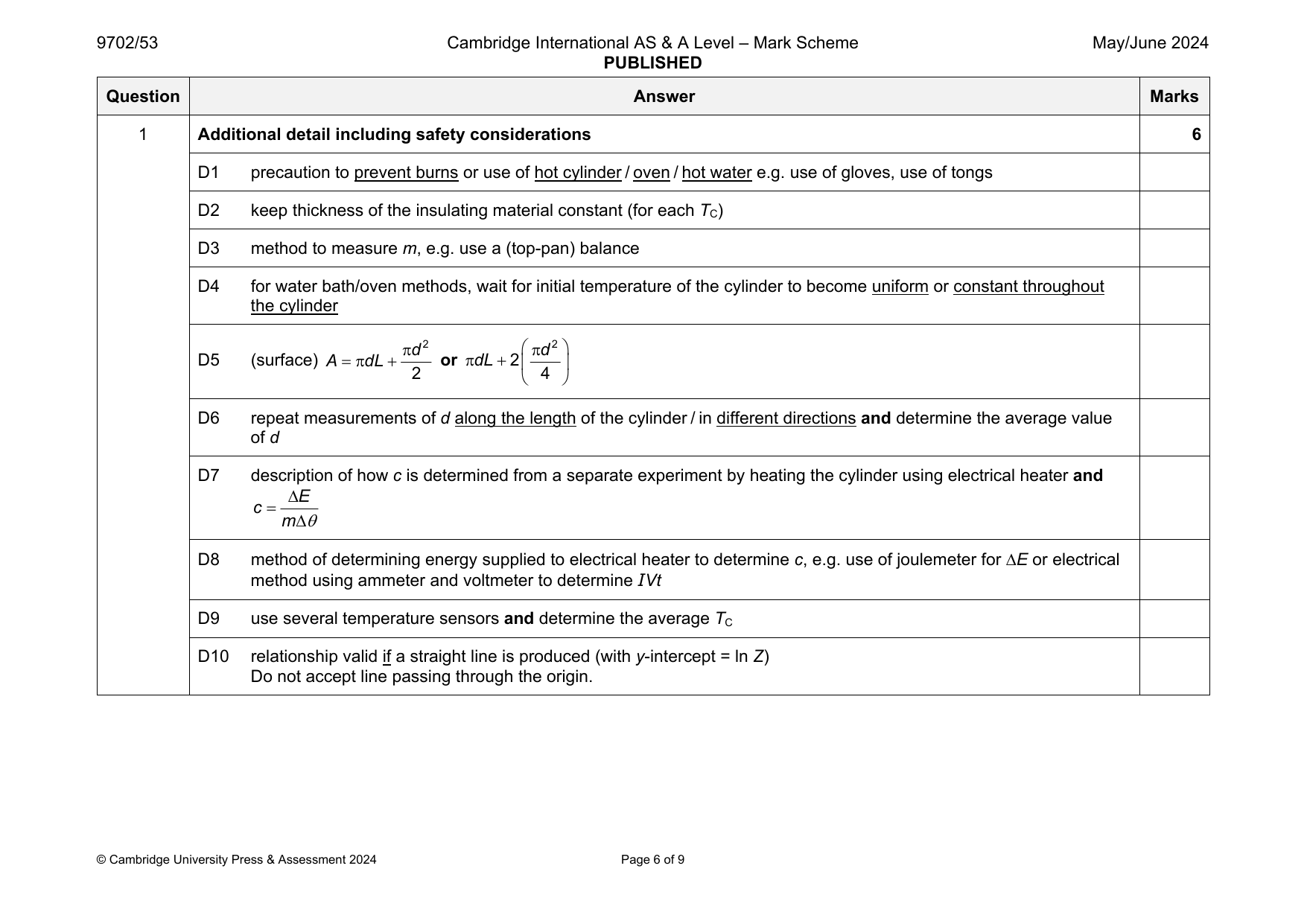
1 Defining the problem
t is the independent variable and T is the dependent variable or vary t and measure T 1
C C
keep T constant 1
R
Methods of data collection
labelled diagram of workable experiment including: 1
solid cylinder cooling
insulation surrounding all of the cylinder
thermometer touching cylinder inside insulation
insulation and thermometer labelled
method to heat the cylinder uniformly, e.g. place in oven/immerse in hot water or diagram showing cylinder in oven or hot 1
water
method to determine time t, e.g. stopwatch or temperature sensor connected to a data logger 1
method to measure L e.g. use a ruler/calipers/micrometer 1
and
method to measure d e.g. use calipers/micrometer
Method of Analysis
plot a graph of ln (T – T ) against t or equivalent 1
C R
mcgradient 1
U
A
Z = ey-intercept 1
© Cambridge University Press & Assessment 2024 Page 5 of 9
1 Additional detail including safety considerations 6
D1 precaution to prevent burns or use of hot cylinder / oven / hot water e.g. use of gloves, use of tongs
D2 keep thickness of the insulating material constant (for each T )
C
D3 method to measure m, e.g. use a (top-pan) balance
D4 for water bath/oven methods, wait for initial temperature of the cylinder to become uniform or constant throughout
the cylinder
d2 d2
D5 (surface) AdL or dL2
Official mark scheme pages: 5, 6 · source PDF URL
9702-2024-mj-53-q02
May/June 2024 · Paper 53 · Question 2 · 15 marks
2 4
D6 repeat measurements of d along the length of the cylinder / in different directions and determine the average value
of d
D7 description of how c is determined from a separate experiment by heating the cylinder using electrical heater and
E
c
m
D8 method of determining energy supplied to electrical heater to determine c, e.g. use of joulemeter for E or electrical
method using ammeter and voltmeter to determine IVt
D9 use several temperature sensors and determine the average T
C
D10 relationship valid if a straight line is produced (with y-intercept = ln Z)
Do not accept line passing through the origin.
© Cambridge University Press & Assessment 2024 Page 6 of 9
2(a) 1 1
gradient =
kf
s
1
y-intercept =
f
s
2(b) 1
1
v / ms–1 / 10–3 Hz–1
f
3.5 0.4 1.118 or 1.1183
6.3 0.4 1.110 or 1.1096
8.7 0.5 1.101 or 1.1013
11.4 0.5 1.092 or 1.0919
13.9 0.6 1.083 or 1.0827
16.2 0.6 1.074 or 1.0739
1
Values of v and correct as shown above.
f
Uncertainties in v correct as shown above. 1
2(c)(i) Six points from (b) plotted correctly. 1
Must be within half a small square. Diameter of points must be less than half a small square.
Error bars in v plotted correctly. 1
All error bars to be plotted. Total length of bar must be accurate to less than half a small square and symmetrical.
© Cambridge University Press & Assessment 2024 Page 7 of 9
2(c)(ii) Straight line of best fit drawn. 1
Do not accept line from top point to bottom point.
Line must pass between (14.5, 1.080) and (14.9, 1.080) and between (4.5, 1.115) and (4.8, 1.115).
Worst acceptable line drawn (steepest or shallowest possible line that passes through all the error bars). 1
All error bars must be plotted.
2(c)(iii) Gradient determined with clear substitution of data points into y / x. 1
Gradient must be negative.
Distance between data points must be greater than half the length of the drawn line.
Gradient determined of worst acceptable line with clear substitution of data points into y / x. 1
uncertainty = (gradient of line of best fit – gradient of worst acceptable line)
or
uncertainty = ½ (steepest worst line gradient – shallowest worst line gradient)
2(c)(iv) y-intercept determined by substitution of correct point with consistent power of ten in m and y into y = mx + c. 1
y-intercept of worst acceptable line determined by substitution into y = mx + c. 1
uncertainty = y-intercept of line of best fit – y-intercept of worst acceptable line
or
uncertainty = ½ (steepest worst line y-intercept – shallowest worst line y-intercept)
Do not accept ECF from false origin method.
© Cambridge University Press & Assessment 2024 Page 8 of 9
2(d)(i) f determined using y-intercept and f given to 2, 3 or 4 significant figures and k given to 2 or 3 significant figures. 1
s s
1
f
s y-intercept
k determined using gradient with method shown and f and k given with SI units with appropriate powers of ten. 1
s
y-intercept 1
k or k
gradient gradientf
s
Units of f : Hz
s
Units of k: m s–1
2(d)(ii) Percentage uncertainty in k with method shown. 1
y-intercept gradient
percentage uncertainty 100
y-intercept gradient
or
correct substitution for max/min methods.
2(e) v determined (non-zero) to a minimum of 2 significant figures from (c)(iii) and (c)(iv) or (d)(i) with correct substitution. 1
1
y-intercept
f
v
gradient
or
kf
v k s
f
© Cambridge University Press & Assessment 2024 Page 9 of 9
Official mark scheme pages: 6, 7, 8, 9 · source PDF URL
9702-2024-on-51-q01
Oct/Nov 2024 · Paper 51 · Question 1 · 15 marks
1 Defining the problem
s is the independent variable and v is the dependent variable or vary s and measure v 1
keep D constant 1
Methods of data collection
labelled diagram of workable experiment including: 1
• light gate positioned at P
• light gate connected to timer / data logger
• labels for light gate and P and data logger / timer and at least one other label from block, magnet(s), trolley, s and D
measure D with a rule(r) and measure L with a rule(r) or calipers 1
description to determine v at P, e.g. (measure length of) card to interrupt beam 1
method to measure s, e.g. use calipers 1
© Cambridge University Press & Assessment 2024 Page 5 of 11
1 Method of Analysis
1 1 1
plot a graph of v2 against or equivalent (e.g. against v2)
s4 s4
Do not accept logarithms.
mgradient 1
K =
2DA2B2L2
m 1
(or K = for against v2)
2DA2B2L2gradient s4
my-intercept 1
Q=−
2D
my-intercept 1
(or Q =KA2B2L2y-intercept or Q = for against v2)
2Dgradient s4
© Cambridge University Press & Assessment 2024 Page 6 of 11
1 Additional detail including safety considerations 6
D1 method to stop the trolley (after passing point P), e.g. labelled block / buffer / cushion drawn after P
or
place a block / buffer / cushion after P to stop the trolley
D2 keep L, A, m and B constant
d2
D3 use micrometer / calipers to measure diameter (d) of the magnet and A =
4
D4 method to secure block to bench, e.g. clamp block to bench or (heavy) mass on top of block
or
method to secure magnets, e.g. use glue to stick magnets to trolley / block
D5 method to increase the accuracy of measuring s or D, e.g. use a marker to left of the trolley
D6 measure B using a (calibrated) Hall probe and adjust / rotate probe until maximum value
or
measure B using Hall probe first in one direction, then in the opposite direction and average
D7 use a (top-pan) balance to measure m
D8 use of strong magnets to increase v
D9 repeat measurements of v for each value of s and average v
2DQ
D10 relationship valid if a straight line is produced (passing through − )
m
Do not accept line passing through the origin.
© Cambridge University Press & Assessment 2024 Page 7 of 11
Official mark scheme pages: 5, 6, 7 · source PDF URL
9702-2024-on-51-q02
Oct/Nov 2024 · Paper 51 · Question 2 · 15 marks
2(a) 3 1
gradient =
3E −E
s
2Z
y-intercept =
3E −E
s
2(b) 1
1
/ A−1
I
5150 or 5155
5560 or 5556
5810 or 5814
6250
6670 or 6667
6940 or 6944
Values correct as shown above.
1 1
Uncertainties in from 50 or 60 to 90 or 100.
I
2(c)(i) Six points from (b) plotted correctly. 1
Must be within half a small square. Diameter of points must be less than half a small square.
1 1
Error bars in plotted correctly.
I
All error bars to be plotted. Total length of bar must be accurate to less than half a small square and symmetrical.
© Cambridge University Press & Assessment 2024 Page 8 of 11
2(c)(ii) Straight line of best fit drawn. 1
Do not accept line from top point to bottom point.
Points must be balanced.
Line must pass between (1.63, 5400) and (1.67, 5400) and between (2.58, 6800) and (2.62, 6800).
Worst acceptable line drawn (steepest or shallowest possible line that passes through all the error bars). 1
All error bars must be plotted.
2(c)(iii) Gradient determined with clear substitution of data points into y / x. 1
Distance between data points must be greater than half the length of the drawn line.
Gradient determined of worst acceptable line with clear substitution of data points into y / x. 1
uncertainty = (gradient of line of best fit – gradient of worst acceptable line)
or
uncertainty = ½ (steepest worst line gradient – shallowest worst line gradient)
2(c)(iv) y-intercept determined by substitution of correct point with consistent power of ten in m and x into y = mx + c. 1
y-intercept of worst acceptable line determined by substitution into y = mx + c. 1
uncertainty = y-intercept of line of best fit – y-intercept of worst acceptable line
or
uncertainty = ½ (steepest worst line y-intercept – shallowest worst line y-intercept)
Do not accept ECF from false origin method.
© Cambridge University Press & Assessment 2024 Page 9 of 11
2(d)(i) E determined using gradient 1
and
E and Z given to 2 or 3 or 4 significant figures.
1 3 3+gradientE 1 E
E = +E = s = + s
3gradient s 3gradient gradient 3
1
E = +0.733
gradient
Z determined using y-intercept 1
and
E and Z given with SI units with correct powers of ten.
(3E −E )y-intercept 3y-intercept
Z = s or Z =
2 2gradient
Unit of E: V
Unit of Z:
2(d)(ii) Absolute uncertainty in E with method shown. 1
gradient 1 0.05
uncertainty= +
gradient gradient 3
or
correct substitution for max/min methods.
© Cambridge University Press & Assessment 2024 Page 10 of 11
2(e) Value of R determined to a minimum of two significant figures from (c)(iii) and (c)(iv) or (d)(i) with correct substitution and 1
correct use of power of ten.
1
−y-intercept
25010−6
R =
gradient
or
1 2Z
R = −
gradient25010−6 3
or
3E −2.2 2Z
R = −
325010−6 3
© Cambridge University Press & Assessment 2024 Page 11 of 11
Official mark scheme pages: 8, 9, 10, 11 · source PDF URL
9702-2024-on-52-q01
Oct/Nov 2024 · Paper 52 · Question 1 · 15 marks
1 Defining the problem
L is the independent variable and or temperature change/increase is the dependent variable 1
or
vary L and measure or temperature change/increase
keep t constant 1
Methods of data collection
labelled diagram of workable experiment including: 1
• oil in a beaker/container (on a bench)
• coil fully submerged in oil
• (bulb of) thermometer in the oil
• at least three labels from thermometer, coil or resistance wire, oil, beaker/container, clamp/stand, bench
Do not accept other heating sources.
method to determine V – diagram of workable circuit including: 1
• power supply connected to wire
• voltmeter positioned to measure V across the coil
measure the initial and final temperature and find the difference 1
method to determine t, e.g. use stopwatch/timer 1
and
method to determine L e.g. use a rule(r) to measure L / length of wire or e.g. using number of turns and measure the
diameter of the coil with rule(r) / calipers
© Cambridge University Press & Assessment 2024 Page 5 of 10
1 Method of Analysis
1 1 1
plot a graph of against or equivalent, e.g. against
L L
Do not accept logarithms.
1
1 1
for against for against
L L
AtV2 AtV2gradient
K = K =
mgradient m
1
1 1
for against for against
L L
Z =−mKy-intercept Z = AtV2y-intercept
or
AtV2y-intercept
Z =−
gradient
© Cambridge University Press & Assessment 2024 Page 6 of 10
1 Additional detail including safety considerations 6
D1 precaution linked to hot oil / beaker / wire, e.g. use of gloves to prevent burns from oil
or
precaution linked to spillage of oil, e.g. perform experiment in a tray
D2 keep A and m and V constant
d2
D3 use a micrometer to measure the diameter (d) of the wire and A =
4
D4 repeat measurements of d along the wire and average
D5 method to reduce heat loss e.g. add insulation around the container / add a lid to the container
D6 method to keep V constant, e.g. adjust / change a variable resistor / power supply to keep V or voltmeter reading
constant
D7 use a balance to determine the mass of the oil
and
mass of oil = mass of (beaker + oil) − mass of beaker
or
place beaker on balance and zero balance, then add oil and read balance
D8 stir the oil for uniform temperature
or
keep the initial temperature (of oil) constant
D9 repeat the experiment for the same value of L and average / average temperature change
Z
D10 relationship valid if a straight line is produced (passing through − )
mK
Do not accept line passing through the origin.
D11 method to determine L accurately, e.g. measure length of unwound coil
© Cambridge University Press & Assessment 2024 Page 7 of 10
Official mark scheme pages: 5, 6, 7 · source PDF URL
9702-2024-on-52-q02
Oct/Nov 2024 · Paper 52 · Question 2 · 15 marks
2(a) gradient = Bn2 1
y-intercept = −B
2(b) 1
d2 / cm2
615 or 615.0
458 or 458.0
292 or 292.4
216 or 216.1
166 or 166.4
139 or 139.2
Values correct as shown above.
Uncertainties in d2 decreasing from 10 to 4 or 5. 1
2(c)(i) Six points from (b) plotted correctly. 1
Must be within half a small square. Diameter of points must be less than half a small square.
Error bars in d2 plotted correctly. 1
All error bars to be plotted. Total length of bar must be accurate to less than half a small square and symmetrical.
2(c)(ii) Straight line of best fit drawn. 1
Do not accept line from top point to bottom point.
Points must be balanced.
Line must pass between (1.90, 250) and (2.00, 250) and between (3.55, 500) and (3.65, 500).
Worst acceptable line drawn (steepest or shallowest possible line that passes through all the error bars). 1
All error bars must be plotted.
© Cambridge University Press & Assessment 2024 Page 8 of 10
2(c)(iii) Gradient determined with clear substitution of data points into y / x. 1
Distance between data points must be greater than half the length of the drawn line.
Gradient determined of worst acceptable line with clear substitution of data points into y / x. 1
uncertainty = (gradient of line of best fit – gradient of worst acceptable line)
or
uncertainty = ½ (steepest worst line gradient – shallowest worst line gradient)
2(c)(iv) y-intercept determined by substitution of correct point with consistent power of ten in m and x into y = mx + c. 1
y-intercept of worst acceptable line determined by substitution into y = mx + c. 1
uncertainty = y-intercept of line of best fit – y-intercept of worst acceptable line
or
uncertainty = ½ (steepest worst line y-intercept – shallowest worst line y-intercept)
Do not accept ECF from false origin method.
2(d)(i) B determined using y-intercept (B = – y-intercept) and B and n given to 2 or 3 or 4 significant figures. 1
n determined using gradient 1
and
B and n given with SI units with correct powers of ten.
gradient gradient
n= or n=
B −y-intercept
Unit for B: cm2
No unit for n.
© Cambridge University Press & Assessment 2024 Page 9 of 10
2(d)(ii) Percentage uncertainty in n determined with method shown. 1
1y-intercept gradient
percentage uncertainty= + 100
2 y-intercept gradient
or
correct substitution for max/min methods.
2(e) determined to a minimum of two significant figures from (c)(iii) and (c)(iv) or (d)(i) with correct substitution and correct 1
power of ten.
gradient
=sin−1
−y-intercept+900
or
n2B
=sin−1
B+900
© Cambridge University Press & Assessment 2024 Page 10 of 10
Official mark scheme pages: 8, 9, 10 · source PDF URL
9702-2024-on-53-q01
Oct/Nov 2024 · Paper 53 · Question 1 · 15 marks
1 Defining the problem
s is the independent variable and v is the dependent variable or vary s and measure v 1
keep D constant 1
Methods of data collection
labelled diagram of workable experiment including: 1
• light gate positioned at P
• light gate connected to timer / data logger
• labels for light gate and P and data logger / timer and at least one other label from block, magnet(s), trolley, s and D
measure D with a rule(r) and measure L with a rule(r) or calipers 1
description to determine v at P, e.g. (measure length of) card to interrupt beam 1
method to measure s, e.g. use calipers 1
© Cambridge University Press & Assessment 2024 Page 5 of 11
1 Method of Analysis
1 1 1
plot a graph of v2 against or equivalent (e.g. against v2)
s4 s4
Do not accept logarithms.
mgradient 1
K =
2DA2B2L2
m 1
(or K = for against v2)
2DA2B2L2gradient s4
my-intercept 1
Q=−
2D
my-intercept 1
(or Q =KA2B2L2y-intercept or Q = for against v2)
2Dgradient s4
© Cambridge University Press & Assessment 2024 Page 6 of 11
1 Additional detail including safety considerations 6
D1 method to stop the trolley (after passing point P), e.g. labelled block / buffer / cushion drawn after P
or
place a block / buffer / cushion after P to stop the trolley
D2 keep L, A, m and B constant
d2
D3 use micrometer / calipers to measure diameter (d) of the magnet and A =
4
D4 method to secure block to bench, e.g. clamp block to bench or (heavy) mass on top of block
or
method to secure magnets, e.g. use glue to stick magnets to trolley / block
D5 method to increase the accuracy of measuring s or D, e.g. use a marker to left of the trolley
D6 measure B using a (calibrated) Hall probe and adjust / rotate probe until maximum value
or
measure B using Hall probe first in one direction, then in the opposite direction and average
D7 use a (top-pan) balance to measure m
D8 use of strong magnets to increase v
D9 repeat measurements of v for each value of s and average v
2DQ
D10 relationship valid if a straight line is produced (passing through − )
m
Do not accept line passing through the origin.
© Cambridge University Press & Assessment 2024 Page 7 of 11
Official mark scheme pages: 5, 6, 7 · source PDF URL
9702-2024-on-53-q02
Oct/Nov 2024 · Paper 53 · Question 2 · 15 marks
2(a) 3 1
gradient =
3E −E
s
2Z
y-intercept =
3E −E
s
2(b) 1
1
/ A−1
I
5150 or 5155
5560 or 5556
5810 or 5814
6250
6670 or 6667
6940 or 6944
Values correct as shown above.
1 1
Uncertainties in from 50 or 60 to 90 or 100.
I
2(c)(i) Six points from (b) plotted correctly. 1
Must be within half a small square. Diameter of points must be less than half a small square.
1 1
Error bars in plotted correctly.
I
All error bars to be plotted. Total length of bar must be accurate to less than half a small square and symmetrical.
© Cambridge University Press & Assessment 2024 Page 8 of 11
2(c)(ii) Straight line of best fit drawn. 1
Do not accept line from top point to bottom point.
Points must be balanced.
Line must pass between (1.63, 5400) and (1.67, 5400) and between (2.58, 6800) and (2.62, 6800).
Worst acceptable line drawn (steepest or shallowest possible line that passes through all the error bars). 1
All error bars must be plotted.
2(c)(iii) Gradient determined with clear substitution of data points into y / x. 1
Distance between data points must be greater than half the length of the drawn line.
Gradient determined of worst acceptable line with clear substitution of data points into y / x. 1
uncertainty = (gradient of line of best fit – gradient of worst acceptable line)
or
uncertainty = ½ (steepest worst line gradient – shallowest worst line gradient)
2(c)(iv) y-intercept determined by substitution of correct point with consistent power of ten in m and x into y = mx + c. 1
y-intercept of worst acceptable line determined by substitution into y = mx + c. 1
uncertainty = y-intercept of line of best fit – y-intercept of worst acceptable line
or
uncertainty = ½ (steepest worst line y-intercept – shallowest worst line y-intercept)
Do not accept ECF from false origin method.
© Cambridge University Press & Assessment 2024 Page 9 of 11
2(d)(i) E determined using gradient 1
and
E and Z given to 2 or 3 or 4 significant figures.
1 3 3+gradientE 1 E
E = +E = s = + s
3gradient s 3gradient gradient 3
1
E = +0.733
gradient
Z determined using y-intercept 1
and
E and Z given with SI units with correct powers of ten.
(3E −E )y-intercept 3y-intercept
Z = s or Z =
2 2gradient
Unit of E: V
Unit of Z:
2(d)(ii) Absolute uncertainty in E with method shown. 1
gradient 1 0.05
uncertainty= +
gradient gradient 3
or
correct substitution for max/min methods.
© Cambridge University Press & Assessment 2024 Page 10 of 11
2(e) Value of R determined to a minimum of two significant figures from (c)(iii) and (c)(iv) or (d)(i) with correct substitution and 1
correct use of power of ten.
1
−y-intercept
25010−6
R =
gradient
or
1 2Z
R = −
gradient25010−6 3
or
3E −2.2 2Z
R = −
325010−6 3
© Cambridge University Press & Assessment 2024 Page 11 of 11
Official mark scheme pages: 8, 9, 10, 11 · source PDF URL
9702-2025-m-52-q01
March 2025 · Paper 52 · Question 1 · 15 marks
1 Defining the problem
Vary p and measure B OR p is the independent variable and B is the dependent variable. 1
Keep V constant or potential difference between the ends of each conductor constant. 1
Methods of data collection
Labelled diagram of workable experiment including: 1
• conductors in parallel connected in series to power supply and resistor
• circuit symbols for (variable) resistor and power supply
• X labelled and one other label from L, P, Q, p and q.
Voltmeter connected in parallel with conductors (to measure V) and conductors in parallel connected to a power supply. 1
Method to measure L and p and q e.g. use a rule / ruler / calipers. 1
Method to measure B, e.g. use a (calibrated) Hall probe and adjust / rotate probe until maximum value. 1
Method of Analysis
1 1
Plots a graph of B against or equivalent.
p
Do not accept logarithms.
1
1 1
B against against B
p p
Lgradient L
Y = Y =
AV AV gradient
© Cambridge University Press & Assessment 2025 Page 7 of 12
1 1
1 1
B against against B
p p
qy-intercept Z =−qy-intercept
Z =
gradient
OR
Lqy-intercept
Z =
YAV
Additional detail including safety considerations 6
Any six from:
D1 precaution linked to high current / hot conductors, e.g. use gloves / switch off power supply when not measuring
B / between measurements / allow conductors to cool
D2 keep A and L and q constant
d2
D3 use calipers / micrometer to measure diameter / d of conductor and A=
4
D4 repeat measurements of d in different positions and average d
D5 method to determine the position of X in relation to the conductors, e.g. divide L by two to find the midpoint of P / Q and
use a set square / protractor / plumb line to mark X
OR
divide L by two to find the midpoint of P / Q and use a grid to mark X
D6 measure B (using Hall probe) first in one direction and then in the opposite direction and average B
OR
Measure B with current / p.d. in one direction and then in the opposite direction and average B
D7 additional detail on measuring p and / or q, e.g. measure to the conductor and add on the radius
© Cambridge University Press & Assessment 2025 Page 8 of 12
1 D8 description of method to keep q constant, e.g. tape / adhesive putty to fix conductor Q to the bench OR for vertical
methods fix conductor Q in clamp(s) attached to stand(s) to keep q constant
D9 method to keep P and Q parallel, e.g. measure the separation (between the conductors) at different points
YZAV
D10 relationship valid if a straight line is produced (with a y-intercept = ).
Lq
Do not accept passing through the origin.
D11 method to keep V constant, e.g. adjust / change variable resistor / power supply to keep voltmeter reading constant.
Question Answer Marks
Official mark scheme pages: 7, 8, 9 · source PDF URL
9702-2025-m-52-q02
March 2025 · Paper 52 · Question 2 · 15 marks
2(a) 1 1
gradient = −
K
y-intercept = ln( − )
0 R
© Cambridge University Press & Assessment 2025 Page 9 of 12
2(b)
( – ) / C ln (( – ) / C)
R R
56.5 1.0 4.034 or 4.0342 0.018
46.0 1.0 3.829 or 3.8286 0.022
38.5 1.0 3.651 or 3.6507 0.026
31.5 1.0 3.450 or 3.4500 0.032
26.0 1.0 3.258 or 3.2581 0.038
22.5 1.0 3.114 or 3.1135 0.044
Values of ( – R) / C and ln (( – R ) / C) 1
Uncertainties in ( – R) and ln (( – R ) / C) 1
2(c)(i) Six points from (b) plotted correctly. 1
Must be within half a small square. Diameter of points must be less than half a small square.
Error bars in ln (( – ) / C) plotted correctly. 1
R
All error bars to be plotted. Total length of bar must be accurate to less than half a small square and symmetrical.
© Cambridge University Press & Assessment 2025 Page 10 of 12
2(c)(ii) Straight line of best fit drawn. 1
Do not accept line from top plot to bottom plot.
Line must pass between
(31.5, 3.2) and (33.0, 3.2) and between
(16.0, 3.7) and (17.0, 3.7)
Worst acceptable line drawn. 1
Steepest or shallowest possible line that passes through all the error bars.
All error bars must be plotted.
2(c)(iii) Gradient must be negative. 1
Gradient determined with clear substitution of data into y / x; distance between data points must be greater than half the
length of the drawn line.
Gradient determined of worst acceptable line with clear substitution of data into y / x; 1
uncertainty = (gradient of line of best fit – gradient of worst acceptable line)
or
uncertainty = ½ (steepest worst line gradient – shallowest worst line gradient)
2(c)(iv) y-intercept determined by substitution of correct point with consistent unit of time into y = mx + c 1
y-intercept of worst acceptable line determined by substitution into y = mx + c. 1
uncertainty = y-intercept of line of best fit – y-intercept of worst acceptable line, or
uncertainty = ½ (steepest worst line y-intercept – shallowest worst line y-intercept)
Do not accept ecf from false origin method.
© Cambridge University Press & Assessment 2025 Page 11 of 12
2(d)(i) K determined using gradient and 1
K and given to 3 or 4 sf.
0
1
K =−
gradient
determined using y-intercept and 1
0
K and
0
given with units with appropriate powers of ten
=ey-intercept +18.5
0
Unit of K: min or minute(s)
unit of : C
0
2(d)(ii) Absolute uncertainty determined with clear method shown. 1
= ( emaxy-intercept +19 ) −(ey-intercept +18.5)
0
OR
= (ey-intercept +18.5)− ( eminy-intercept +18 )
0
OR
( emaxy-intercept +19 ) − ( eminy-intercept +18 )
=
0 2
2(e) t determined to a minimum of 2sf from (c)(iii) and (c)(iv) OR (d)(i) with correct substitution and correct power of ten. 1
ln(25.0−18.5)−y-intercept
t =
gradient
OR
t =−K(ln(25.0−18.5)−y-intercept)
OR
25.0−18.5
t =−Kln
−18.5
0
© Cambridge University Press & Assessment 2025 Page 12 of 12
Official mark scheme pages: 9, 10, 11, 12 · source PDF URL
9702-2025-mj-51-q01
May/June 2025 · Paper 51 · Question 1 · 15 marks
1 Defining the problem
vary f and measure V or f is the independent variable and V is the dependent variable 1
keep E constant 1
Methods of data collection
labelled diagram of workable experiment including: 1
• circuit with a.c. supply
• oscilloscope connected in parallel with the resistor
• workable circuit
• oscilloscope and a.c. supply labelled
labelled signal generator or variable frequency power supply connected across the terminals 1
method to determine V or E from oscilloscope, e.g. multiply amplitude / height of wave by y-gain on oscilloscope 1
method to determine f from oscilloscope, e.g. determine period T by multiplying number of divisions in 1 cycle or horizontal 1
distance in 1 cycle by the time base and f = 1/T
Method of Analysis
1 1 1
plot a graph of against f or equivalent, e.g. f against
V V
Allow logarithms e.g. lg V against lg f.
relationship valid if a straight line is produced passing through the origin 1
(for lg V against lg f: relationship valid if a straight line is produced with gradient = −1)
© Cambridge University Press & Assessment 2025 Page 7 of 12
1 1
1 1
against f f against
V V
lES lES 1
K = gradient K =
AN2 AN2 gradient
ElS
(for lg V against lg f: K = 10−y-intercept).
AN2
Additional detail including safety considerations 6
D1 precaution linked to hot coil or hot resistor or prevention of burns from coil or resistor, e.g. use gloves / switch off
power supply when not measuring V to prevent burns from coil / resistor
D2 keep N and A and l and S constant
D3 method to keep S constant, e.g. switch off power supply between readings to prevent heating of resistor or to allow
resistor to cool
d2
D4 method to determine A, e.g. use calipers / micrometer to measure diameter (of coil) / d and A=
4
D5 repeat measurements of diameter d along the length of the coil / in different directions and determine the average
value of d
D6 method to determine the value of S, e.g. separate circuit diagram showing resistor connected to ohmmeter, or
circuit diagram showing resistor connected to a power supply with an ammeter and voltmeter and S = V / I
D7 measure l with a ruler / calipers
D8 oscilloscope drawn connected across terminals / across signal generator and description to determine E
D9 adjust y-gain for maximum amplitude
or
adjust time base for length of one wave or measure n waves and divide measured time by n
© Cambridge University Press & Assessment 2025 Page 8 of 12
1 D10 method to keep E constant, e.g. check p.d. and alter supply
or
method to keep l constant, e.g. tape coil
or
method to keep A constant, e.g. wind wire on a cylinder
Question Answer Marks
Official mark scheme pages: 7, 8, 9 · source PDF URL
9702-2025-mj-51-q02
May/June 2025 · Paper 51 · Question 2 · 15 marks
2(a) R 1
gradient =
E
Z
y-intercept =
E
2(b) 1
1
/ 103 A–1
I
2.20 or 2.198
1.90 or 1.905
1.72 or 1.724
1.57 or 1.575
1.46 or 1.460
1.31 or 1.307
1
Values of / 103 A–1 correct as shown above.
I
© Cambridge University Press & Assessment 2025 Page 9 of 12
2(b) 1 1
Uncertainties in / 103 A–1 from 0.02 or 0.03 decreasing to 0.01.
I
2(c)(i) Six points from (b) plotted correctly. 1
Must be within half a small square. Diameter of points must be less than half a small square.
1 1
Error bars in plotted correctly.
I
All error bars to be plotted. Total length of bar must be accurate to less than half a small square and symmetrical.
2(c)(ii) Straight line of best fit drawn. 1
Thickness of the line must be less than half a small square.
Do not accept line from top point to bottom point.
Line must pass between (0.101, 1.40) and (0.104, 1.40) and between (0.189, 2.10) and (0.194, 2.10)
Worst acceptable straight line drawn (steepest or shallowest possible line that passes through all the error bars). 1
Thickness of the line must be less than half a small square.
All error bars must be plotted.
2(c)(iii) Gradient determined with clear substitution of data points into y / x. 1
Distance between data points must be greater than half the length of the drawn line.
Gradient determined of worst acceptable line with clear substitution of data points into y / x. 1
uncertainty = (gradient of line of best fit – gradient of worst acceptable line)
or
uncertainty = ½ (steepest worst line gradient – shallowest worst line gradient)
© Cambridge University Press & Assessment 2025 Page 10 of 12
2(c)(iv) y-intercept determined by substitution of correct point with consistent power of ten in m and y into y = mx + c. 1
y-intercept of worst acceptable line determined by substitution into y = mx + c. 1
uncertainty = y-intercept of line of best fit – y-intercept of worst acceptable line
or
uncertainty = ½ (steepest worst line y-intercept – shallowest worst line y-intercept)
Do not accept ECF from false origin method.
2(d)(i) R determined using gradient and R and Z given to 2 or 3 significant figures. 1
R = gradient 5.8
Z determined using y-intercept and R and Z given with units with appropriate powers of ten. 1
Z = y-intercept 5.8
unit of R: or V A–1
unit of Z: or V A–1
2(d)(ii) Percentage uncertainty determined using E = 0.2 (V) with method shown. 1
E gradient
R%= + 100
E gradient
or
0.2 gradient
R%= + 100
5.8 gradient
© Cambridge University Press & Assessment 2025 Page 11 of 12
2(e) I determined to a minimum of 2 significant figures from (c)(iii) and (c)(iv) or (d)(i) with correct substitution. 1
1
I =
gradient
+y-intercept
20
or
E
I =
R
+Z
20
© Cambridge University Press & Assessment 2025 Page 12 of 12
Official mark scheme pages: 9, 10, 11, 12 · source PDF URL
9702-2025-mj-52-q01
May/June 2025 · Paper 52 · Question 1 · 15 marks
1 Defining the problem
vary m and measure v or m is the independent variable and v is the dependent variable 1
keep h constant 1
Methods of data collection
labelled diagram of workable experiment including: 1
• axle resting on support(s) (on stands)
• supports placed on bench
• light gate (connected to timer) positioned at a distance h
• light gate labelled and h indicated
vertical metre rule clamped to a stand in a position close to block to measure h 1
method to determine v using an interrupt length, e.g. v = length of block / time recorded by the timer 1
method to measure m, e.g. use a (top-pan) balance 1
Method of analysis
1 1 1
plot a graph of against or equivalent
v2 m
Do not accept logarithms.
© Cambridge University Press & Assessment 2025 Page 7 of 12
1 1
1 1 1 1
against against
v2 m m v2
1 gradient
P = P =−
hy-intercept y-intercepth
or
r2zgradient
P =
2Qh
1
1 1 1 1
against against
v2 m m v2
r2z r2zy-intercept
Q= Q=−
2Phgradient 2
or
r2zy-intercept
Q=
2gradient
Additional detail including safety considerations 6
D1 precaution linked to falling block resulting in damage to block / bench, e.g. use a cushion / sand tray to prevent
damage to bench
or
precaution linked to stands falling, e.g. clamp stand(s) to the bench prevent stand falling
D2 keep r and z constant
D3 method to determine r e.g. use calipers / ruler to measure diameter d and r = d / 2
D4 measure z with a micrometer / calipers
© Cambridge University Press & Assessment 2025 Page 8 of 12
1 D5 set square correctly positioned between rule and bench to ensure that rule to measure h is vertical
D6 method to keep h constant by identifying constant initial position of the bottom of the block, e.g. clamped pin / rod to
indicate the starting point each time or (fiducial) marker on rule
D7 description of method to ensure that axle can rotate, e.g. axle is lubricated at the supports to enable axle to rotate,
axle is not fixed at the supports so axle can rotate
D8 use a large length of block to reduce (percentage) uncertainty in interrupt time or increase the time light gate is
interrupted
D9 repeat experiment for the same value of m and determine the average v
1
D10 relationship valid if a straight line is produced (with y-intercept = ).
hP
Do not accept line passing through the origin.
© Cambridge University Press & Assessment 2025 Page 9 of 12
Official mark scheme pages: 7, 8, 9 · source PDF URL
9702-2025-mj-52-q02
May/June 2025 · Paper 52 · Question 2 · 15 marks
2(a) C 1
gradient =
EA
1
y-intercept =
E
2(b) 1
1
V/ V / V–1
V
4.25 0.235 or 0.2353
3.70 0.270 or 0.2703
3.25 0.308 or 0.3077
2.90 0.345 or 0.3448
2.60 0.385 or 0.3846
2.35 0.426 or 0.4255
1
Values of V / V and / V–1 correct as shown above.
V
Uncertainties in V all 0.05 1
and
1
uncertainties in from 0.002 or 0.003 increasing to 0.009.
V
© Cambridge University Press & Assessment 2025 Page 10 of 12
2(c)(i) Six points from (b) plotted correctly. 1
Must be within half a small square. Diameter of points must be less than half a small square.
1 1
Error bars in plotted correctly.
V
All error bars must be plotted. Total length of bar must be accurate to less than half a small square and symmetrical.
2(c)(ii) Straight line of best fit drawn. 1
Thickness of the line must be less than half a small square.
Do not accept line from top point to bottom point.
Line must pass between (2.65, 0.26) and (2.80, 0.26) and between (6.30, 0.40) and (6.50, 0.40).
Worst acceptable straight line drawn (steepest or shallowest possible line that passes through all the error bars). 1
Thickness of the line must be less than half a small square.
All error bars must be plotted.
2(c)(iii) Gradient determined with clear substitution of data points into y / x. 1
Distance between data points must be greater than half the length of the drawn line.
Gradient determined of worst acceptable line with clear substitution of data points into y / x. 1
uncertainty = (gradient of line of best fit – gradient of worst acceptable line)
or
uncertainty = ½ (steepest worst line gradient – shallowest worst line gradient)
2(c)(iv) y-intercept determined by substitution of correct point into y = mx + c. 1
y-intercept of worst acceptable line determined by substitution into y = mx + c. 1
uncertainty = y-intercept of line of best fit – y-intercept of worst acceptable line
or
uncertainty = ½ (steepest worst line y-intercept – shallowest worst line y-intercept)
Do not accept ECF from false origin method.
© Cambridge University Press & Assessment 2025 Page 11 of 12
2(d)(i) E determined using y-intercept and E and C given to 2 or 3 significant figures. 1
1
E =
y-intercept
C determined using gradient and E and C given with correct units with appropriate powers of ten. 1
Agradient
C = or C=AEgradient
y-intercept
unit of E: V
unit of C: F
2(d)(ii) Percentage uncertainty determined with method shown. 1
A gradient y-intercept
C%= + + 100
A gradient y-intercept
or
A gradient E
C%= + + 100 with method to determine E shown
A gradient E
2(e) V determined to a minimum of 2 significant figures from (c)(iii) and (c)(iv) or (d)(i) with correct substitution. 1
1
V =
10gradient+y-intercept
or
EA
V =
10C +A
© Cambridge University Press & Assessment 2025 Page 12 of 12
Official mark scheme pages: 10, 11, 12 · source PDF URL
9702-2025-mj-53-q01
May/June 2025 · Paper 53 · Question 1 · 15 marks
1 Defining the problem
vary f and measure V or f is the independent variable and V is the dependent variable 1
keep E constant 1
Methods of data collection
labelled diagram of workable experiment including: 1
• circuit with a.c. supply
• oscilloscope connected in parallel with the resistor
• workable circuit
• oscilloscope and a.c. supply labelled
labelled signal generator or variable frequency power supply connected across the terminals 1
method to determine V or E from oscilloscope, e.g. multiply amplitude / height of wave by y-gain on oscilloscope 1
method to determine f from oscilloscope, e.g. determine period T by multiplying number of divisions in 1 cycle or horizontal 1
distance in 1 cycle by the time base and f = 1/T
Method of Analysis
1 1 1
plot a graph of against f or equivalent, e.g. f against
V V
Allow logarithms e.g. lg V against lg f.
relationship valid if a straight line is produced passing through the origin 1
(for lg V against lg f: relationship valid if a straight line is produced with gradient = −1)
© Cambridge University Press & Assessment 2025 Page 7 of 12
1 1
1 1
against f f against
V V
lES lES 1
K = gradient K =
AN2 AN2 gradient
ElS
(for lg V against lg f: K = 10−y-intercept).
AN2
Additional detail including safety considerations 6
D1 precaution linked to hot coil or hot resistor or prevention of burns from coil or resistor, e.g. use gloves / switch off
power supply when not measuring V to prevent burns from coil / resistor
D2 keep N and A and l and S constant
D3 method to keep S constant, e.g. switch off power supply between readings to prevent heating of resistor or to allow
resistor to cool
d2
D4 method to determine A, e.g. use calipers / micrometer to measure diameter (of coil) / d and A=
4
D5 repeat measurements of diameter d along the length of the coil / in different directions and determine the average
value of d
D6 method to determine the value of S, e.g. separate circuit diagram showing resistor connected to ohmmeter, or
circuit diagram showing resistor connected to a power supply with an ammeter and voltmeter and S = V / I
D7 measure l with a ruler / calipers
D8 oscilloscope drawn connected across terminals / across signal generator and description to determine E
D9 adjust y-gain for maximum amplitude
or
adjust time base for length of one wave or measure n waves and divide measured time by n
© Cambridge University Press & Assessment 2025 Page 8 of 12
1 D10 method to keep E constant, e.g. check p.d. and alter supply
or
method to keep l constant, e.g. tape coil
or
method to keep A constant, e.g. wind wire on a cylinder
Question Answer Marks
Official mark scheme pages: 7, 8, 9 · source PDF URL
9702-2025-mj-53-q02
May/June 2025 · Paper 53 · Question 2 · 15 marks
2(a) R 1
gradient =
E
Z
y-intercept =
E
2(b) 1
1
/ 103 A–1
I
2.20 or 2.198
1.90 or 1.905
1.72 or 1.724
1.57 or 1.575
1.46 or 1.460
1.31 or 1.307
1
Values of / 103 A–1 correct as shown above.
I
© Cambridge University Press & Assessment 2025 Page 9 of 12
2(b) 1 1
Uncertainties in / 103 A–1 from 0.02 or 0.03 decreasing to 0.01.
I
2(c)(i) Six points from (b) plotted correctly. 1
Must be within half a small square. Diameter of points must be less than half a small square.
1 1
Error bars in plotted correctly.
I
All error bars to be plotted. Total length of bar must be accurate to less than half a small square and symmetrical.
2(c)(ii) Straight line of best fit drawn. 1
Thickness of the line must be less than half a small square.
Do not accept line from top point to bottom point.
Line must pass between (0.101, 1.40) and (0.104, 1.40) and between (0.189, 2.10) and (0.194, 2.10)
Worst acceptable straight line drawn (steepest or shallowest possible line that passes through all the error bars). 1
Thickness of the line must be less than half a small square.
All error bars must be plotted.
2(c)(iii) Gradient determined with clear substitution of data points into y / x. 1
Distance between data points must be greater than half the length of the drawn line.
Gradient determined of worst acceptable line with clear substitution of data points into y / x. 1
uncertainty = (gradient of line of best fit – gradient of worst acceptable line)
or
uncertainty = ½ (steepest worst line gradient – shallowest worst line gradient)
© Cambridge University Press & Assessment 2025 Page 10 of 12
2(c)(iv) y-intercept determined by substitution of correct point with consistent power of ten in m and y into y = mx + c. 1
y-intercept of worst acceptable line determined by substitution into y = mx + c. 1
uncertainty = y-intercept of line of best fit – y-intercept of worst acceptable line
or
uncertainty = ½ (steepest worst line y-intercept – shallowest worst line y-intercept)
Do not accept ECF from false origin method.
2(d)(i) R determined using gradient and R and Z given to 2 or 3 significant figures. 1
R = gradient 5.8
Z determined using y-intercept and R and Z given with units with appropriate powers of ten. 1
Z = y-intercept 5.8
unit of R: or V A–1
unit of Z: or V A–1
2(d)(ii) Percentage uncertainty determined using E = 0.2 (V) with method shown. 1
E gradient
R%= + 100
E gradient
or
0.2 gradient
R%= + 100
5.8 gradient
© Cambridge University Press & Assessment 2025 Page 11 of 12
2(e) I determined to a minimum of 2 significant figures from (c)(iii) and (c)(iv) or (d)(i) with correct substitution. 1
1
I =
gradient
+y-intercept
20
or
E
I =
R
+Z
20
© Cambridge University Press & Assessment 2025 Page 12 of 12
Official mark scheme pages: 9, 10, 11, 12 · source PDF URL
9702-2025-on-51-q01
Oct/Nov 2025 · Paper 51 · Question 1 · 15 marks
1 Defining the problem
vary r and measure v or r is the independent variable and v is the dependent variable 1
keep x constant 1
Methods of data collection
labelled diagram of workable experiment including: 1
• one end of spring resting against block clamped to bench using G-clamp
• light gate positioned at P
• light gate connected to timer
• apparatus shown on bench
• labels for light gate and P and at least one other label from bench, block, stand, spring, ball, timer
method to determine r, e.g. use calipers or micrometer to measure diameter d and r = d / 2 1
description of method to determine v, use diameter of ball (to interrupt beam) ÷ measured time at light gate positioned at P 1
instrument to determine x, e.g. rule(r) or calipers 1
Method of Analysis
plot a graph of (2 lg v) or (lg v2) against lg r 1
or
plot a graph of (lg v) against (lg r) or equivalent, e.g. (ln v) against (ln r)
n=−gradient for (2 lg v) or (lg v2) against lg r 1
or
n=−2gradient for (lg v) against lg r
© Cambridge University Press & Assessment 2025 Page 7 of 11
1 10y-intercept 1
Y = for (2 lg v) or (lg v2) against lg r
kx2
or
102y-intercept
Y = for (lg v) against lg r
kx2
Additional detail including safety considerations 6
D1 precaution to prevent ball leaving bench, e.g. screens around apparatus / cushions on bench (to stop the ball)
D2 keep k and constant
D3 description of method to determine k, e.g. add mass to spring and k = mg / extension
or
use newton meter to measure force applied to spring and k = force / extension
or
take several readings of force and extension, plot a force–extension graph and k = gradient
m
D4 description of experimental method to determine , e.g. measure mass of ball using a balance and =
4
r3
3
D5 repeat measurements of diameter or d in different directions and determine the average value of d
D6 method to keep x constant, e.g. use a pin / ruler / card to indicate the starting point each time to keep x constant
D7 x = original length of spring – compressed length of spring
D8 adjust (vertical) position of light gate so that the diameter of (each) ball cuts the beam
D9 repeat experiment for the same value of r and determine the average v
© Cambridge University Press & Assessment 2025 Page 8 of 11
1 Ykx2 1 Ykx2
D10 relationship valid if a straight line is produced (with y-intercept = lg or lg ).
2
Do not accept line through the origin.
Question Answer Marks
Official mark scheme pages: 7, 8, 9 · source PDF URL
9702-2025-on-51-q02
Oct/Nov 2025 · Paper 51 · Question 2 · 15 marks
2(a) gradient = H 1
0
y-intercept =
0
2(b) 1
d
/ 1015s
c
(1.6 or 1.60) 0.40
(3.47 or 3.467) 0.40
(4.83 or 4.833) 0.40
(6.00 or 6.000) 0.40
(9.50 or 9.500) 0.40
(12.5 or 12.50) 0.40
d
Values of correct as shown above.
c
d 1
Uncertainties in correct as shown above.
c
© Cambridge University Press & Assessment 2025 Page 9 of 11
2(c)(i) Six points from (b) plotted correctly. 1
Must be within half a small square. Diameter of points must be less than half a small square.
d 1
Error bars in plotted correctly.
c
All error bars must be plotted. Total length of bar must be accurate to less than half a small square and symmetrical.
2(c)(ii) Straight line of best fit drawn. 1
Thickness of the line must be less than half a small square.
Do not accept line from top point to bottom point.
Line must pass between (2.5, 660.0) and (2.9, 660.0) and between (11.2, 676.0) and (11.6, 676.0).
Worst acceptable line drawn (steepest or shallowest possible line that passes through all the error bars). 1
Thickness of the line must be less than half a small square.
All error bars must be plotted.
2(c)(iii) Gradient determined with clear substitution of data points into y / x. 1
Distance between data points must be greater than half the length of the drawn line.
Gradient determined of worst acceptable line with clear substitution of data points into y / x. 1
uncertainty = (gradient of line of best fit – gradient of worst acceptable line)
or
uncertainty = ½ (steepest worst line gradient – shallowest worst line gradient)
2(c)(iv) y-intercept determined by substitution of correct point with consistent power of ten in m and x and y into y = mx + c. 1
y-intercept of worst acceptable line determined by substitution into y = mx + c. 1
uncertainty = y-intercept of line of best fit – y-intercept of worst acceptable line
or
uncertainty = ½ (steepest worst line y-intercept – shallowest worst line y-intercept)
Do not accept ECF from false origin method.
© Cambridge University Press & Assessment 2025 Page 10 of 11
2(d) determined using y-intercept and given to 3 or 4 significant figures and H given to 2, 3 or 4 significant figures. 1
0 0
= y-intercept
0
H determined using gradient and and H given with SI units with appropriate powers of ten. 1
0
gradient gradient
H = or H =
y-intercept
0
Unit of : m, nm, m
0
Unit of H: s−1
2(e) Value of T determined to a minimum of two significant figures from (d) and correct power of ten. 1
1
T =
H
Absolute uncertainty determined with correct substitution. 1
y-intercept gradient
T = + T
y-intercept gradient
or
max maxy-intercept
T = 0 −T or T = −T
min gradient min gradient
or
min miny-intercept
T = 0 −T or T = −T
max gradient max gradient
© Cambridge University Press & Assessment 2025 Page 11 of 11
Official mark scheme pages: 9, 10, 11 · source PDF URL
9702-2025-on-52-q01
Oct/Nov 2025 · Paper 52 · Question 1 · 15 marks
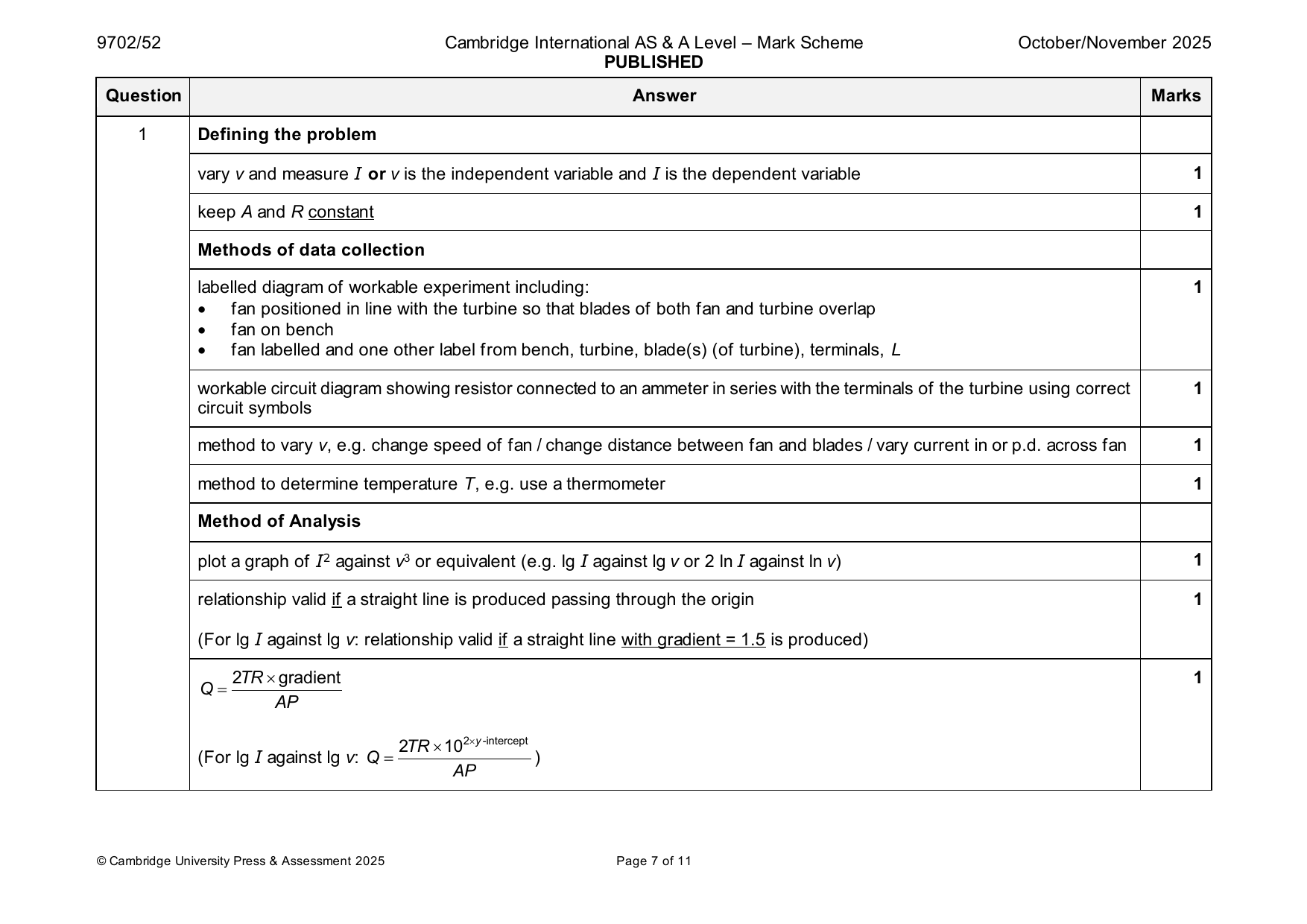
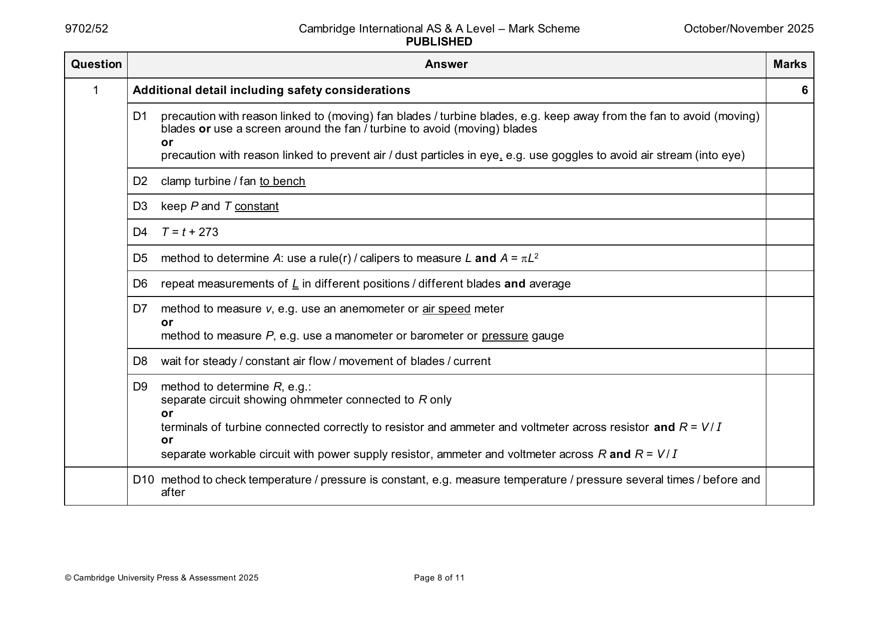
1 Defining the problem
vary v and measure I or v is the independent variable and I is the dependent variable 1
keep A and R constant 1
Methods of data collection
labelled diagram of workable experiment including: 1
• fan positioned in line with the turbine so that blades of both fan and turbine overlap
• fan on bench
• fan labelled and one other label from bench, turbine, blade(s) (of turbine), terminals, L
workable circuit diagram showing resistor connected to an ammeter in series with the terminals of the turbine using correct 1
circuit symbols
method to vary v, e.g. change speed of fan / change distance between fan and blades / vary current in or p.d. across fan 1
method to determine temperature T, e.g. use a thermometer 1
Method of Analysis
plot a graph of I2 against v3 or equivalent (e.g. lg I against lgv or 2 lnI against lnv) 1
relationship valid if a straight line is produced passing through the origin 1
(For lg I against lg v: relationship valid if a straight line with gradient = 1.5 is produced)
2TRgradient 1
Q=
AP
2TR102y-intercept
(For lg I against lg v: Q = )
AP
© Cambridge University Press & Assessment 2025 Page 7 of 11
1 Additional detail including safety considerations 6
D1 precaution with reason linked to (moving) fan blades / turbine blades, e.g. keep away from the fan to avoid (moving)
blades or use a screen around the fan / turbine to avoid (moving) blades
or
precaution with reason linked to prevent air / dust particles in eye, e.g. use goggles to avoid air stream (into eye)
D2 clamp turbine / fan to bench
D3 keep P and T constant
D4 T = t + 273
D5 method to determine A: use a rule(r) / calipers to measure L and A = L2
D6 repeat measurements of L in different positions / different blades and average
D7 method to measure v, e.g. use an anemometer or air speed meter
or
method to measure P, e.g. use a manometer or barometer or pressure gauge
D8 wait for steady / constant air flow / movement of blades / current
D9 method to determine R, e.g.:
separate circuit showing ohmmeter connected to R only
or
terminals of turbine connected correctly to resistor and ammeter and voltmeter across resistor and R = V / I
or
separate workable circuit with power supply resistor, ammeter and voltmeter across R and R = V / I
D10 method to check temperature / pressure is constant, e.g. measure temperature / pressure several times / before and
after
© Cambridge University Press & Assessment 2025 Page 8 of 11
Official mark scheme pages: 7, 8 · source PDF URL
9702-2025-on-52-q02
Oct/Nov 2025 · Paper 52 · Question 2 · 15 marks
2(a) gradient = n 1
2
y-intercept = lg
k
2(b) 1
lg (r / 108 m) lg (T / 103 s)
0.152 or 0.1523 (1.72 or 1.716) 0.04
0.270 or 0.2695 (1.91 or 1.908) 0.03
0.377 or 0.3766 (2.08 or 2.079 or 2.0792) 0.04
0.470 or 0.4698 (2.23 or 2.230 or 2.2304) 0.03
0.576 or 0.5763 (2.38 or 2.380 or 2.3802) 0.04
0.723 or 0.7226 (2.59 or 2.591 or 2.5911) 0.03
Values of lg (r / 108 m) and lg (T / 103 s) correct as shown above.
Uncertainties in lg (T / 103 s) correct as shown above. 1
2(c)(i) Six points from (b) plotted correctly. 1
Must be within half a small square. Diameter of points must be less than half a small square.
Error bars in lg (T / 103 s) plotted correctly. 1
All error bars must be plotted. Total length of bar must be accurate to less than half a small square and symmetrical.
© Cambridge University Press & Assessment 2025 Page 9 of 11
2(c)(ii) Straight line of best fit drawn. 1
Thickness of the line must be less than half a small square.
Do not accept line from top point to bottom point.
Line must pass between (0.19, 1.80) and (0.21, 1.80) and between (0.645, 2.50) and (0.66, 2.50).
Worst acceptable line drawn (steepest or shallowest possible line that passes through all the error bars). 1
Thickness of the line must be less than half a small square.
All error bars must be plotted.
2(c)(iii) Gradient determined with clear substitution of data points into y / x. 1
Distance between data points must be greater than half the length of the drawn line.
Gradient determined of worst acceptable line with clear substitution of data points into y / x. 1
uncertainty = (gradient of line of best fit – gradient of worst acceptable line)
or
uncertainty = ½ (steepest worst line gradient – shallowest worst line gradient)
2(c)(iv) y-intercept determined by substitution of correct point with consistent powers of ten into y = mx + c. 1
y-intercept of worst acceptable line determined by substitution into y = mx + c. 1
uncertainty = y-intercept of line of best fit – y-intercept of worst acceptable line
or
uncertainty = ½ (steepest worst line y-intercept – shallowest worst line y-intercept)
Do not accept ECF from false origin method.
© Cambridge University Press & Assessment 2025 Page 10 of 11
2(d) Value of n determined using gradient and n and k given to 2 or 3 significant figures. 1
n=gradient=(c)(iii)
Value of k determined using y-intercept. 1
Correct method must be seen.
2 2
k = =
10y-intercept 10(c)(iv)
Absolute uncertainties in n and k determined. 1
Absolute uncertainty in n = absolute uncertainty in gradient
and
2 2
k = −
10y-intercept 10WAL y-intercept
Correct method must be seen.
2(e) r determined to a minimum of 2 significant figures from (c)(iii) and (c)(iv) or (d) with correct substitution and correct power 1
of ten.
lg1380−y-intercept
r =10 gradient 108
or
k1380
r = n 108
2π
© Cambridge University Press & Assessment 2025 Page 11 of 11
Official mark scheme pages: 9, 10, 11 · source PDF URL
9702-2025-on-53-q01
Oct/Nov 2025 · Paper 53 · Question 1 · 15 marks
1 Defining the problem
vary r and measure v or r is the independent variable and v is the dependent variable 1
keep x constant 1
Methods of data collection
labelled diagram of workable experiment including: 1
• one end of spring resting against block clamped to bench using G-clamp
• light gate positioned at P
• light gate connected to timer
• apparatus shown on bench
• labels for light gate and P and at least one other label from bench, block, stand, spring, ball, timer
method to determine r, e.g. use calipers or micrometer to measure diameter d and r = d / 2 1
description of method to determine v, use diameter of ball (to interrupt beam) ÷ measured time at light gate positioned at P 1
instrument to determine x, e.g. rule(r) or calipers 1
Method of Analysis
plot a graph of (2 lg v) or (lg v2) against lg r 1
or
plot a graph of (lg v) against (lg r) or equivalent, e.g. (ln v) against (ln r)
n=−gradient for (2 lg v) or (lg v2) against lg r 1
or
n=−2gradient for (lg v) against lg r
© Cambridge University Press & Assessment 2025 Page 7 of 11
1 10y-intercept 1
Y = for (2 lg v) or (lg v2) against lg r
kx2
or
102y-intercept
Y = for (lg v) against lg r
kx2
Additional detail including safety considerations 6
D1 precaution to prevent ball leaving bench, e.g. screens around apparatus / cushions on bench (to stop the ball)
D2 keep k and constant
D3 description of method to determine k, e.g. add mass to spring and k = mg / extension
or
use newton meter to measure force applied to spring and k = force / extension
or
take several readings of force and extension, plot a force–extension graph and k = gradient
m
D4 description of experimental method to determine , e.g. measure mass of ball using a balance and =
4
r3
3
D5 repeat measurements of diameter or d in different directions and determine the average value of d
D6 method to keep x constant, e.g. use a pin / ruler / card to indicate the starting point each time to keep x constant
D7 x = original length of spring – compressed length of spring
D8 adjust (vertical) position of light gate so that the diameter of (each) ball cuts the beam
D9 repeat experiment for the same value of r and determine the average v
© Cambridge University Press & Assessment 2025 Page 8 of 11
1 Ykx2 1 Ykx2
D10 relationship valid if a straight line is produced (with y-intercept = lg or lg ).
2
Do not accept line through the origin.
Question Answer Marks
Official mark scheme pages: 7, 8, 9 · source PDF URL
9702-2025-on-53-q02
Oct/Nov 2025 · Paper 53 · Question 2 · 15 marks
2(a) gradient = H 1
0
y-intercept =
0
2(b) 1
d
/ 1015s
c
(1.6 or 1.60) 0.40
(3.47 or 3.467) 0.40
(4.83 or 4.833) 0.40
(6.00 or 6.000) 0.40
(9.50 or 9.500) 0.40
(12.5 or 12.50) 0.40
d
Values of correct as shown above.
c
d 1
Uncertainties in correct as shown above.
c
© Cambridge University Press & Assessment 2025 Page 9 of 11
2(c)(i) Six points from (b) plotted correctly. 1
Must be within half a small square. Diameter of points must be less than half a small square.
d 1
Error bars in plotted correctly.
c
All error bars must be plotted. Total length of bar must be accurate to less than half a small square and symmetrical.
2(c)(ii) Straight line of best fit drawn. 1
Thickness of the line must be less than half a small square.
Do not accept line from top point to bottom point.
Line must pass between (2.5, 660.0) and (2.9, 660.0) and between (11.2, 676.0) and (11.6, 676.0).
Worst acceptable line drawn (steepest or shallowest possible line that passes through all the error bars). 1
Thickness of the line must be less than half a small square.
All error bars must be plotted.
2(c)(iii) Gradient determined with clear substitution of data points into y / x. 1
Distance between data points must be greater than half the length of the drawn line.
Gradient determined of worst acceptable line with clear substitution of data points into y / x. 1
uncertainty = (gradient of line of best fit – gradient of worst acceptable line)
or
uncertainty = ½ (steepest worst line gradient – shallowest worst line gradient)
2(c)(iv) y-intercept determined by substitution of correct point with consistent power of ten in m and x and y into y = mx + c. 1
y-intercept of worst acceptable line determined by substitution into y = mx + c. 1
uncertainty = y-intercept of line of best fit – y-intercept of worst acceptable line
or
uncertainty = ½ (steepest worst line y-intercept – shallowest worst line y-intercept)
Do not accept ECF from false origin method.
© Cambridge University Press & Assessment 2025 Page 10 of 11
2(d) determined using y-intercept and given to 3 or 4 significant figures and H given to 2, 3 or 4 significant figures. 1
0 0
= y-intercept
0
H determined using gradient and and H given with SI units with appropriate powers of ten. 1
0
gradient gradient
H = or H =
y-intercept
0
Unit of : m, nm, m
0
Unit of H: s−1
2(e) Value of T determined to a minimum of two significant figures from (d) and correct power of ten. 1
1
T =
H
Absolute uncertainty determined with correct substitution. 1
y-intercept gradient
T = + T
y-intercept gradient
or
max maxy-intercept
T = 0 −T or T = −T
min gradient min gradient
or
min miny-intercept
T = 0 −T or T = −T
max gradient max gradient
© Cambridge University Press & Assessment 2025 Page 11 of 11
Official mark scheme pages: 9, 10, 11 · source PDF URL